DARK FIRESORIGINS UNKNOWN

Author: Dark Fires

  • Testing a Planet Identification with JPL Horizons

    Testing a Planet Identification with JPL Horizons

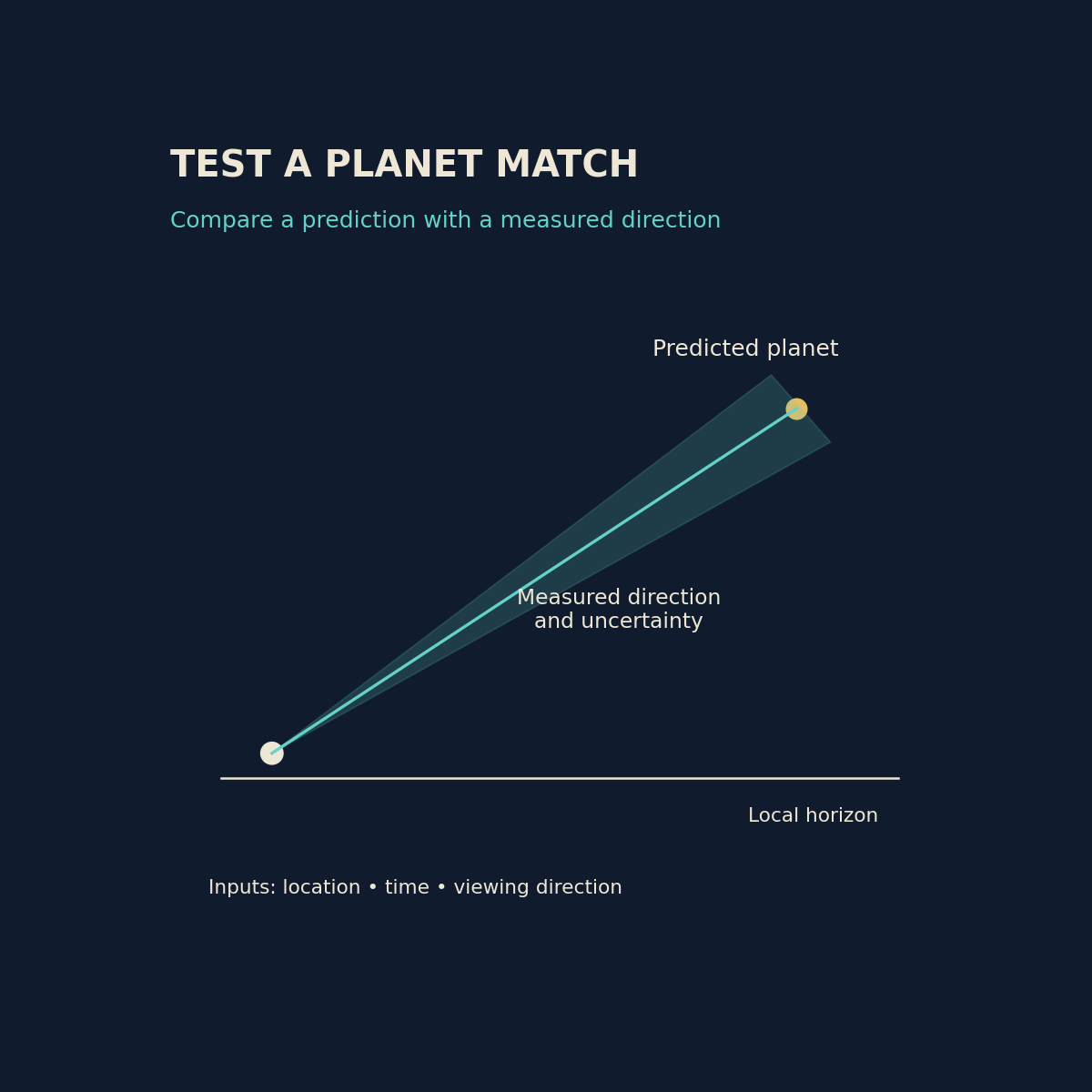
    Original diagram by Dark Fires. Schematic, not an observation; not to scale.

    A bright light reported in the same part of the sky over several minutes deserves a check against known astronomical objects. A planet identification becomes useful when it predicts the observation’s direction and timing, rather than merely naming a bright object that happened to be visible that night.

    Build the prediction from the observer’s position

    NASA JPL’s Horizons tutorial describes observer tables for the apparent observing quantities of solar-system bodies. For a terrestrial sighting, choose the candidate body, the observer’s geographical location and a time interval covering the report. A prediction from Earth’s centre is not the same setup as a prediction for a specific observer.

    Preserve the entered coordinates, height, date, time scale and output settings. Convert the witness’s local civil time carefully, including daylight-saving rules where applicable. If “about nine” could mean a range of times, calculate the range. A precisely printed table cannot repair an uncertain input.

    Compare direction before appearance

    Azimuth describes direction around the horizon and elevation describes angle above it. The Horizons manual documents observer quantities and atmospheric-refraction options. Confirm the conventions in the output instead of guessing which direction corresponds to zero degrees or whether refraction has already been included.

    Use a landmark, a surveyed camera position or recognizable stars to constrain the recorded direction. Treat an uncalibrated phone compass as an estimate. Buildings and terrain can obscure a predicted object even when its calculated elevation is above a mathematical horizon. A sky application screenshot is helpful only when its location, time and orientation are also preserved.

    Compare the full sequence. Does the candidate occupy the reported sector at the beginning and end? Is its slow change of direction consistent with the footage? Does it disappear behind the same obstruction? Agreement across several independent constraints is more informative than a resemblance in colour or brightness.

    Avoid forcing a match

    Consider a hypothetical report placing a light between 220 and 230 degrees azimuth. A candidate predicted at 225 degrees fits that rough direction; one at 290 degrees does not become a good match merely because it is bright. This example illustrates a test, not an identification of any actual case.

    Horizons concerns solar-system targets. It is not a general catalogue for identifying every star, aircraft or artificial Earth satellite in a video. If a planetary candidate fails, document that failure and choose the appropriate tool for another class of source rather than stretching the result.

    State what the comparison establishes

    Publish the saved query settings and relevant output beside the measured direction and its uncertainty. Use language such as “consistent with Venus within the available timing and bearing uncertainty” when that is what the evidence supports. A strong astronomical match can explain a sighting, but the mere presence of a planet somewhere above the horizon cannot.
    Sources and further reading

  • MTG-I2’s First Images Preview a Faster Watch on Europe’s Weather

    MTG-I2’s First Images Preview a Faster Watch on Europe’s Weather

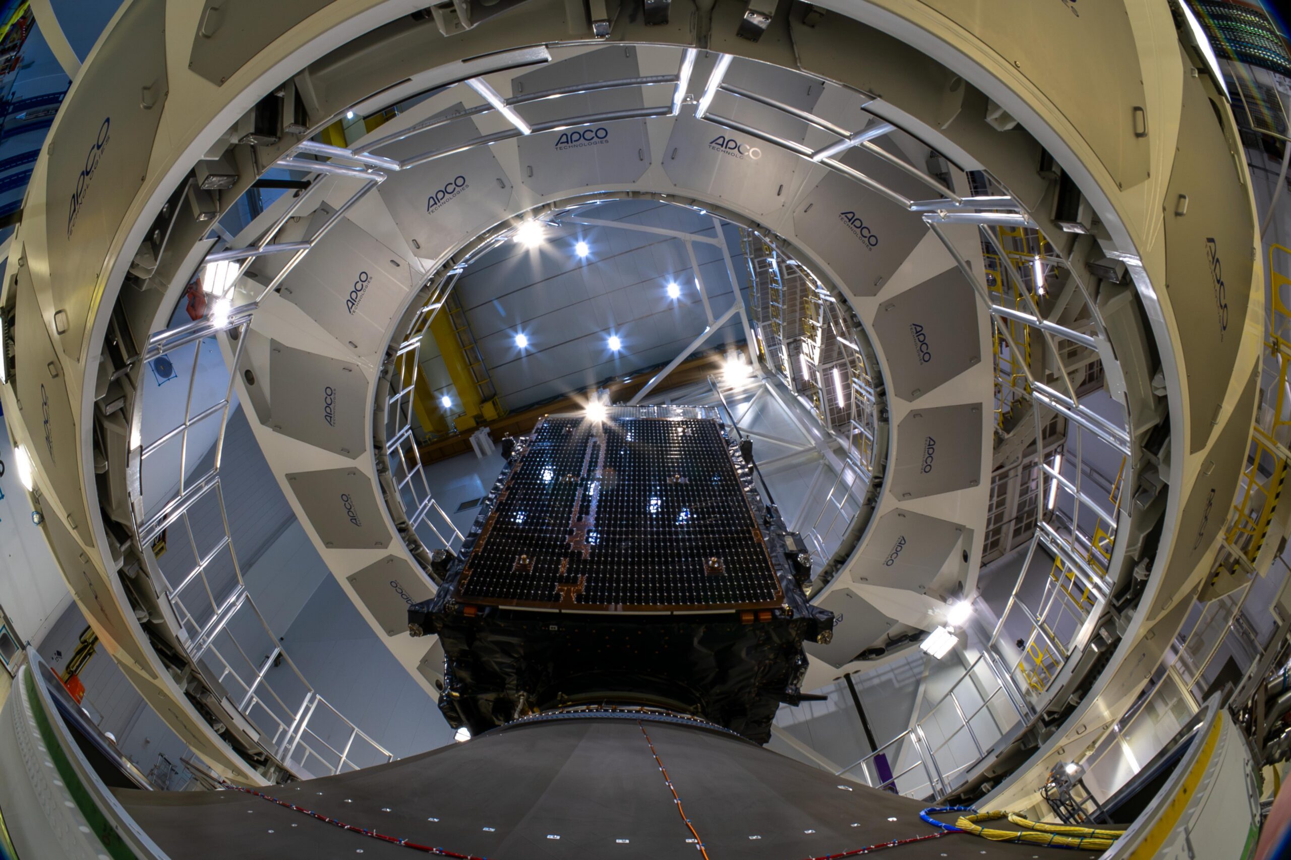
    MTG-I2 during encapsulation at Europe’s Spaceport on 21 August 2026, before launch. Photo: ©ESA – M. Pédoussaut. Image source.

    Europe’s newest weather imager has begun showing what a faster view of the atmosphere can reveal. ESA released the first MTG-I2 imagery on 6 November 2026, previewing a satellite service designed to revisit Europe and North Africa every two and a half minutes.

    The release includes a 45-hour sequence beginning on 3 November. It shows persistent fog over central Europe, developing Mediterranean clouds and a wildfire smoke plume in Portugal. The rapid regional coverage will complement the first MTG Imager’s ten-minute views of a full Earth hemisphere.

    There is an important commissioning step still ahead. MTG-I2 remains in calibration and validation, with operational service expected in the second quarter of 2027. The pictures demonstrate emerging capability, rather than announcing that the new service is already part of routine forecasting. ESA’s first-images announcement sets out that distinction.

    From launch to a working observatory

    The new release follows an orbital handover that ESA described in September. After separating from its Ariane 6 launcher, MTG-I2 needed a sequence of engine burns to reach its geostationary position at 3.5 degrees east. Teams also deployed antennas and turned the satellite toward Earth before commissioning could begin.

    EUMETSAT took over the spacecraft on 8 September. Its existing companions are MTG-I1, launched in 2022, and the MTG-S1 sounder, launched in 2025. An industrial team led by Thales Alenia Space, working with OHB and Leonardo, developed the constellation with ESA and EUMETSAT. EUMETSAT operates the system. ESA’s orbital-arrival account explains the work between launch and instrument checkout.

    Why the time between pictures matters

    The practical significance of the faster cadence is easiest to understand as a sampling problem. A single image records a situation; successive images reveal how that situation changes. Shortening the gap gives forecasters more opportunities to distinguish growth, movement and dissipation. That is particularly relevant when the subject of interest is evolving within a larger cloud field.

    It also helps explain why regional and hemispheric observations serve different purposes. A broad view supplies context, while frequent revisits concentrate attention on a smaller area. The two products can be complementary without offering identical coverage or timing.

    The next test of this promise will be the completed operational service. Attractive first images are a useful milestone, but users ultimately need dependable measurements, repeatable processing and a clear understanding of data quality. For now, the release provides an early look at the pace of observation Europe is preparing to add.

  • Twining’s 1947 Flying-Disc Memorandum: A Call to Investigate, Not a Verdict

    Twining’s 1947 Flying-Disc Memorandum: A Call to Investigate, Not a Verdict

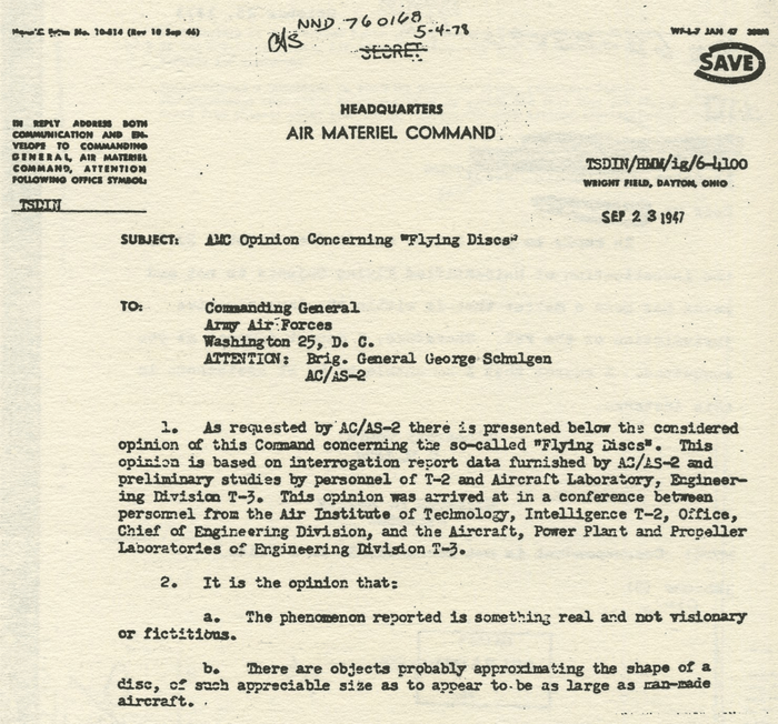
    Image: Cropped detail of the first page of the 23 September 1947 Twining memorandum. The full letter includes qualifications and a recommendation for further study. Credit: U.S. Air Force, via Wikimedia Commons. Public domain, U.S. federal government work Full first-page scan and image source.

    On 23 September 1947, Lieutenant General Nathan F. Twining signed an Air Materiel Command assessment of reported flying discs. Its best-known sentence described the reported phenomenon as “something real and not visionary or fictitious.” Reading that sentence alone, however, removes the document’s uncertainty and its practical purpose.

    What kind of record is this?

    The memorandum was addressed to Army Air Forces headquarters, for the attention of Brigadier General George Schulgen. It presented a command opinion based on interrogation reports and preliminary technical work. It summarized reported appearances and performance, considered natural phenomena, and raised both domestic and foreign technological possibilities. Crucially, it acknowledged a lack of recovered physical exhibits that would conclusively establish the objects’ existence. Its recommendation was a dedicated study with information shared among relevant scientific and military bodies. Read the memorandum reproduced as Appendix R of the government-sponsored Colorado study.

    This is therefore an assessment of a reporting problem. It is not a laboratory report on recovered material, a description of an inspected vehicle, or a statement that its origin had been established. Those are different documentary categories, and substituting one for another changes what the evidence says.

    The importance of conditional language

    The letter repeatedly works with possibilities and estimates. That does not make it meaningless. An intelligence organization may reasonably recommend investigation before it has a complete explanation. Indeed, the threshold for deciding that reports deserve attention should be lower than the threshold for declaring a revolutionary discovery.

    The reverse mistake is also possible: treating every expression of uncertainty as proof that the authors had dismissed the reports. The recommendation to establish a more organized inquiry is plainly incompatible with simple indifference. The document shows that officers regarded the subject as worth technical attention, while remaining short of a demonstrated explanation.

    How to test a claim about the memo

    A useful reading method is to ask three questions. Is a passage reporting what witnesses described, offering an institutional judgment, or recommending future work? Does a later retelling retain the qualifying words? Finally, does the conclusion being advertised actually appear in the document?

    For example, unusual reported maneuvering and a proven propulsion system are not equivalent propositions. Likewise, considering a secret domestic project does not demonstrate that such a project existed. Listing a foreign technological possibility does not identify a foreign manufacturer. Each stronger claim would require evidence beyond this letter.

    The first-page scan is useful for checking the opening language against later quotations, but the remaining pages are essential to understanding the argument. A cropped sentence should never stand in for the complete recommendation.

    Twining’s memorandum remains important because it captures an early official attempt to turn uncertain aerial reports into a researchable problem. Its historical value does not depend on converting that uncertainty into a conclusion the authors had not reached. The strongest reading is also the most restrained: investigate systematically, compare possibilities, and recognize the missing physical evidence.

  • The Battle of Los Angeles: What the 1942 Military History Actually Says

    The Battle of Los Angeles: What the 1942 Military History Actually Says

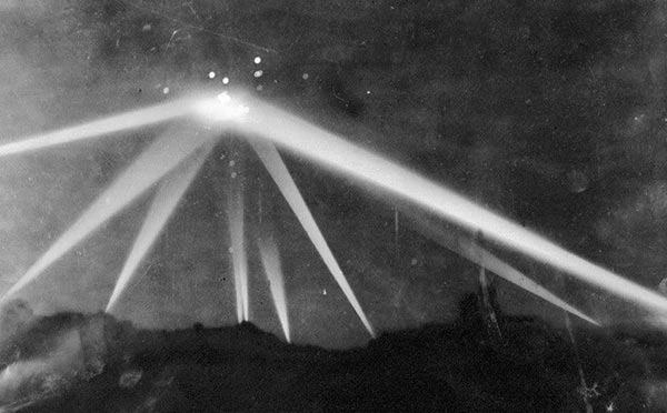
    Image: Searchlights during the Los Angeles air-raid alarm of February 1942. The photograph does not establish the presence of a solid craft. Credit: Unknown photographer / Associated Press, via Wikimedia Commons. Public domain in United States: published 1931–1963 without copyright renewal, per Commons rights statement. Other jurisdictions may differ. Image source.

    In the early hours of 25 February 1942, antiaircraft guns opened fire above Los Angeles. The shooting was real. Whether the defenders had identified an aircraft was another question. That distinction is central to understanding an episode later absorbed into UFO history.

    An alarm in a vulnerable city

    The official Army Air Forces history places the incident after a Japanese submarine shelled installations at Ellwood on 23 February. It describes a radar warning, a regional blackout at 2:21 a.m., and increasingly inconsistent reports. A balloon carrying a red flare was reported over Santa Monica at 3:06 a.m. The history records 1,440 rounds fired, no enemy losses, and no bombs dropped. Navy Secretary Frank Knox called the episode a false alarm; the Army initially entertained aircraft explanations. These are findings and reported observations in a retrospective government history, not a surviving instrument record demonstrating an extraordinary vehicle. Read the official history, pages 282–286, reproduced by HyperWar.

    What the later assessment proposed

    The same account suggests meteorological balloons may have started the alarm and describes shell bursts and drifting smoke complicating observation. That wording matters: it proposes a reconstruction rather than supplying a positively identified object for every report. Its footnotes point back to wartime command histories, messages and contemporary newspapers. The accessible edition therefore lets readers distinguish the historians’ explanation from the reports they evaluated.

    There is a common logical trap here. If soldiers fired at a reported target, that establishes a military response. It does not establish that every estimate of the target’s shape, distance or speed was accurate. Nor does the absence of a downed aircraft demonstrate that an object possessed an impenetrable surface. A claim of invulnerability requires evidence that a physical target was present and struck, not simply that ammunition was expended.

    Reading the photograph cautiously

    The familiar searchlight photograph is an important artifact of the event. It records an illuminated night sky and the public spectacle of the barrage. It cannot, on its own, identify the material at the intersection of the beams. A bright patch in a photograph must not automatically become a solid craft in the caption. The archived image and its provenance should travel with any reproduction.

    The most useful unresolved questions are narrow: what initiated particular alerts, which observations were independent, and how much later reporting repeated earlier impressions. Those questions invite comparison of dated records. They do not require choosing between a flawless military explanation and an extraterrestrial visitation.

    Los Angeles belongs in the history of unidentified aerial reports because it shows how uncertainty can become an operational emergency. The surviving account supports a serious failure of identification under wartime pressure. It does not provide verified evidence of a nonhuman aircraft. Keeping those conclusions separate preserves both the event’s historical importance and the limits of its evidence.

  • Digital Zoom and UAP Evidence: Bigger Pixels Are Not New Measurements

    Digital Zoom and UAP Evidence: Bigger Pixels Are Not New Measurements

    Original diagram by Dark Fires. Schematic, not an observation; not to scale.

    A light can fill a phone screen while still being represented by very little independent scene information. Zoom labels describe an imaging operation, not a guarantee that an object’s surface or outline has been resolved. For UAP analysis, the useful question is what detail reached the sensor before enlargement and processing.

    Separate optical capture from enlargement

    Optical zoom changes the image formed by the lens. Standard digital zoom enlarges information already captured. Sony’s documentation distinguishes conventional digital enlargement from other branded zoom modes and explains that ordinary digital zoom estimates additional image signals. Those estimates can make a picture easier to inspect without providing the same evidence as additional optical sampling.

    The exact pipeline matters. A phone may switch lenses, crop a higher-resolution sensor, combine frames or apply computational enhancement as a zoom slider moves. Do not assume every enlargement behaves identically. Record the device, camera application, selected lens, capture mode and original image dimensions. A simple on-screen “10×” label is insufficient to reconstruct that history.

    A hypothetical pixel example

    Imagine a distant source covering only three original pixels across. Enlarging the picture fourfold can display that source across twelve output pixels. The larger display makes the original sample pattern easier to see, but the extra output pixels are not twelve separate measurements across the source. A smooth border may be interpolation, and a crisp-looking rim may depend on processing.

    This does not mean enlargement is useless. It can help locate a source, compare frames or show a feature already present in the original. The evidential problem starts when a processed enlargement is treated as proof of windows, panels, appendages or a precise silhouette that cannot be demonstrated in the underlying samples.

    A reproducible inspection method

    Begin with the untouched original at native resolution. Make separate, clearly labeled copies for enlargement. Compare a nearest-neighbour display, which exposes the pixel grid, with a conventional smooth enlargement. Neither becomes a ground-truth photograph; the comparison simply reveals how strongly the apparent shape depends on the display method.

    Keep a record of crop boundaries, scaling factor and enhancement settings. If software reconstructs or generates plausible detail, label the result as an interpretation and exclude it from measurements of unobserved structure. Do not place a reconstructed illustration beside the original without a prominent explanation of the difference.

    For a continuing observation, prioritize a stable original recording and optical capture where available. Sony’s zoom guidance recommends optical-only settings when prioritizing image quality. This is practical camera advice, not a promise that optical zoom will resolve every distant light.

    A defensible conclusion

    Report the source’s original pixel extent, the enlargement method and which features persist without enhancement. If the object remains unresolved, say so. A large image can be useful evidence of a light’s presence while remaining weak evidence of its physical construction.

    Sources and further reading

  • When a Point Becomes a Streak: Exposure Time in UAP Images

    When a Point Becomes a Streak: Exposure Time in UAP Images

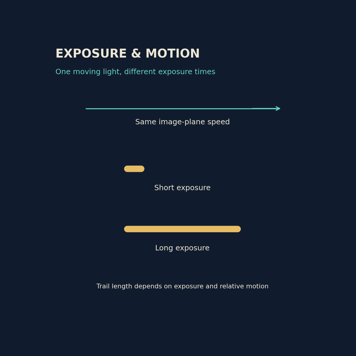
    Original diagram by Dark Fires. Schematic, not an observation; not to scale.

    A luminous streak in a photograph records light collected over an interval. Its length can reflect movement during that interval rather than the length of a solid object. Before interpreting a bright bar, hook or ribbon as an aircraft structure, establish how long the camera was collecting light and whether the camera itself moved.

    What the camera measures

    Nikon’s shutter-speed guide explains that longer exposures admit light for longer and make motion blur more likely. The relevant movement is movement across the sensor. A stationary distant light can trace a path when a handheld camera shakes; a moving source can leave a trail even on a tripod.

    Exposure time and frame rate are different quantities. A video marked 30 frames per second describes how often frames are delivered, not necessarily the exposure duration of each frame. Obtain the actual setting or camera metadata instead of assuming that every frame was exposed for exactly one thirtieth of a second.

    A small calculation with strict limits

    Consider a hypothetical point whose image moves at 120 pixels per second across a fixed camera sensor. During a one-tenth-second exposure, its ideal motion trail spans about 12 pixels. During a one-hundredth-second exposure, it spans about 1.2 pixels. This simple calculation assumes steady motion, constant image scale and uninterrupted exposure. It does not convert pixels into metres or establish the object’s speed through space.

    The same limitation applies in reverse. Dividing trail length by exposure time estimates image-plane motion only when the trail really comes from motion and the timing is known. Focus, optical spreading, clipping and processing can widen or reshape a trail. A clipped social-media video may not preserve enough information to separate those contributions.

    A practical comparison

    Keep the original file and inspect nearby stars, distant lamps or other references. Similar hooks on several unrelated lights support camera movement as a shared cause. A sharp background with one elongated source supports relative source motion, though it still does not identify the source. These are comparisons to test, not automatic verdicts.

    If an observation continues, record a stable wide view and then, where practical, a shorter exposure without changing the viewpoint. Note every settings change. Basler’s imaging guidance recommends short enough exposure that a moving image does not travel more than roughly one pixel when blur must be minimized. In a dark sky this may make the source faint, so preserve both versions.

    How to report the result

    Write that a source produced a measured trail during a stated exposure, and list camera-motion uncertainty. Reserve claims about physical shape or acceleration for evidence that survives those checks. An exposure explanation can account for a strange image without identifying the light that produced it.

    Sources and further reading

  • Four NASA Cameras Trace November 5 Fireball Across the Tennessee Region

    Four NASA Cameras Trace November 5 Fireball Across the Tennessee Region

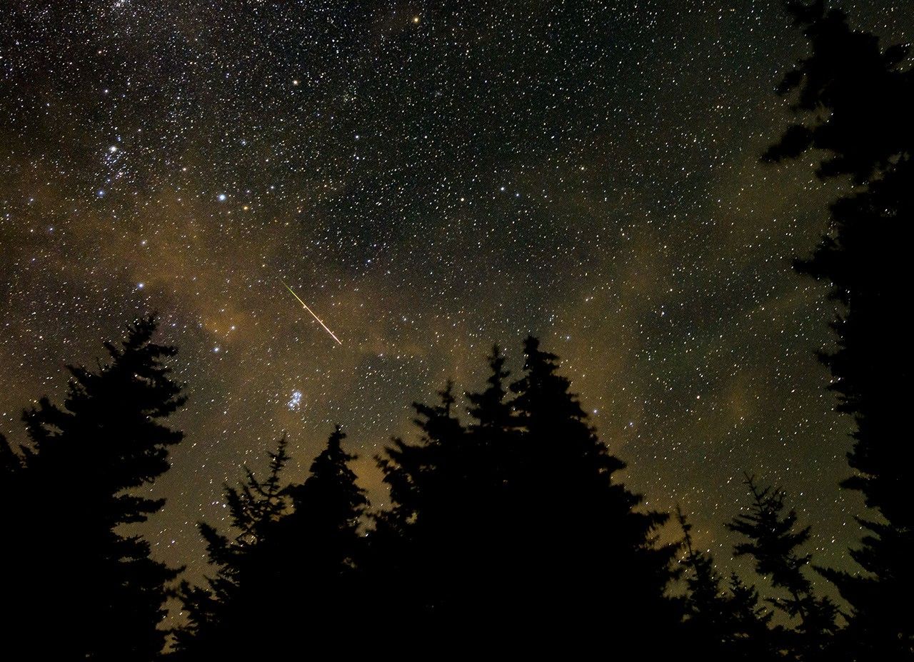
    Context photograph: a Perseid meteor over West Virginia in August 2021, photographed by NASA’s Bill Ingalls. This is not the November 5, 2026 Tennessee event.

    A bright meteor reported over southern Tennessee on November 5, 2026, was recorded by four NASA all-sky cameras. The agency’s analysis identifies a small asteroid fragment and explicitly rules out membership in the active Taurid meteor shower.

    NASA’s event record places the observation at 7:45 p.m. Eastern Standard Time, or 6:45 p.m. Central. Its precise timestamp is November 6 at 00:45:21 UTC. The different calendar dates describe the same event, an important detail when matching recordings and witness accounts.

    A measured path above two states

    The object first appeared above Robbinsville, North Carolina, moving slightly south of west. NASA says it disintegrated above East Ridge, Tennessee, southeast of Chattanooga. The event table gives a camera-observed altitude range of 86.3 to 40.5 kilometers, and a speed of 21.2 kilometers per second, approximately 47,500 miles per hour.

    The agency estimates the incoming fragment was about two inches across and weighed six ounces. These are estimates of the small body responsible for the luminous event, not measurements of a recovered rock. The record does not announce a meteorite recovery.

    Why the shower label matters

    A meteor appearing during a shower’s active period does not automatically belong to that shower. Here the classification comes from NASA’s event analysis, which directly states that this fireball was not a Taurid. Calendar proximity should not replace that finding in descriptions of the footage.

    NASA’s background explanation of fireballs describes how atmospheric entry converts part of a meteoroid’s kinetic energy into visible light. A striking flash therefore does not require an object comparable in size to the bright area seen in a camera frame. The light records an energetic interaction with the atmosphere.

    This case also illustrates the difference between a widely shared clip and a documented event. A useful comparison begins with time, observing location and viewing direction, then asks whether a recording matches the measured passage. A dramatic appearance alone cannot establish that two videos show the same object.

    The photograph accompanying this article is an older NASA image of a Perseid meteor in West Virginia, used only for context. It is not a photograph of the Tennessee fireball and should not be circulated as evidence of this event.

    Featured image: NASA/Bill Ingalls. Perseid meteor photographed in West Virginia on August 11, 2021; contextual photograph, NOT the November 5, 2026 Tennessee fireball. Public domain. Image source.

  • Misty Moons Uses a Cosmic Lens to Expose Compact Star Formation in an Early Galaxy

    Misty Moons Uses a Cosmic Lens to Expose Compact Star Formation in an Early Galaxy

    A distant galaxy nicknamed Misty Moons offers a close look at a normally inaccessible question: how much of an early galaxy’s stellar mass was concentrated in small, bright clumps rather than spread smoothly through it?

    The study, highlighted in November 6 coverage after publication in The Astrophysical Journal on October 19, uses gravitational lensing to examine a galaxy estimated to lie at redshift 11 to 12. This is not a discovery first announced this weekend: the team’s preprint initially appeared in November 2025 and was revised in July 2026.

    Several images of one galaxy

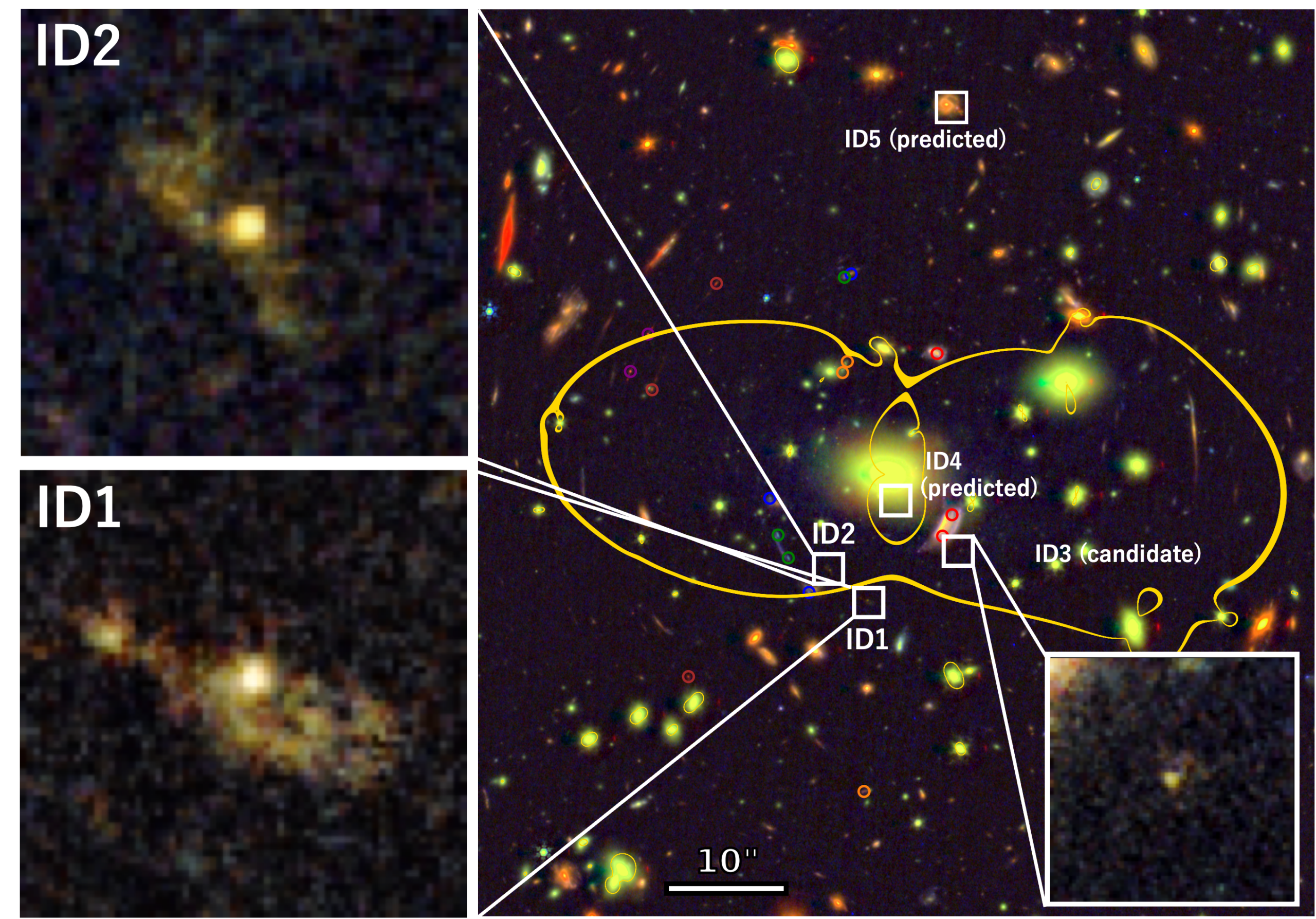
    The foreground galaxy cluster MACS J0257.1-2325 bends the light traveling toward Earth. Two bright images of Misty Moons are magnified roughly 20 to 30 times, allowing Webb to reveal internal features that would otherwise blend together.

    Two independent lens models predict five images of the same background galaxy. The analysis concentrates on the two brightest, with a third candidate identified and two others below detection. Multiple images are useful because the reconstructed source should have a consistent structure even when the foreground lens stretches each view differently.

    The researchers estimate that individual stellar clumps have effective radii of roughly 10 to 70 parsecs and masses around ten million Suns. Together, the clumps account for at least about 80 percent of the inferred stellar mass. That concentration points to a clustered form of early star formation.

    Where the uncertainties enter

    The redshift is estimated from imaging through different filters, rather than established by a spectroscopic measurement in this analysis. It places the object approximately 370 million to 410 million years after the Big Bang under the study’s cosmological interpretation. The exact physical picture also depends on correcting for lens magnification and fitting models to the observed light.

    As the November report explains, the bright central structures may include light from an accreting black hole. Such a contribution would complicate estimates that attribute the light to stars. The possible connection between these clumps and the ancestors of globular clusters is consequently a research question rather than a demonstrated evolutionary history.

    The larger value of Misty Moons is that a natural lens opens its internal structure to scrutiny. An ordinary unresolved image can make several star-forming knots look like one compact object. Here, astronomers can begin asking which pieces create the apparent brightness, and test those answers against more than one view of the same galaxy.

    Featured image: Minami Nakane et al., VENUS collaboration (2026), Figure 1; JWST/NIRCam and Hubble observations. CC BY 4.0. Image source; license.

  • Salt-Loving Microbes Grow Under Combined Mars-Like Stresses in a Laboratory Test

    Salt-Loving Microbes Grow Under Combined Mars-Like Stresses in a Laboratory Test

    A salt-loving Earth microorganism has grown during a 160-day experiment combining several stresses relevant to possible shallow habitats on Mars. The result strengthens a laboratory method for studying habitability while leaving a central planetary question open: whether a suitable environment actually exists there.

    The study, published November 5, 2026, in Applied and Environmental Microbiology, tested Haloferax volcanii, an archaeon. Researchers maintained cultures in salty liquid under oxygen-free, carbon-dioxide-rich conditions at 24 millibars, far below ordinary terrestrial atmospheric pressure. Cultures received nitrate or perchlorate as alternative electron acceptors for metabolism.

    Separating survival from growth

    Being recoverable after exposure to a hostile setting is different from multiplying within it. The researchers used changes in optical density, together with chemical measurements of nitrate and perchlorate reduction, to assess activity. Cultures without the added compounds showed no significant increase in optical density, providing a comparison against the growing treatments.

    Growth at low pressure was lower than in comparable Earth-pressure cultures. Electron microscopy also revealed biofilms in the growing low-pressure treatments, while the liquid lost less than four percent of its volume over the experiment. These observations give future studies several measurable outcomes beyond a simple alive-or-dead result.

    The limits of the simulated habitat

    The University of Florida’s account of the work emphasizes two important advantages the organisms received: a temperature of about 21 degrees Celsius and nutrients provided by the researchers. Much of the Martian subsurface is considerably colder. The proposed liquid-water pockets motivating the experiment have not been confirmed on Mars.

    Those qualifications define what the result can support. It demonstrates that this terrestrial organism can grow under a particular combination of laboratory conditions. It cannot establish that those conditions occur together naturally, persist long enough, or contain the necessary food on another planet.

    The experiment also has a practical connection to spacecraft cleanliness. Knowing which microbes can remain active under combinations of planetary stresses helps researchers assess contamination risks, as well as design instruments to look for biological activity.

    For life-detection research, the useful next question is which constraints change the outcome. Temperature, nutrient availability and the stability of liquid water each need to be tested alongside the stresses already combined here. A laboratory success becomes more informative when its boundaries are mapped as carefully as its favorable result.

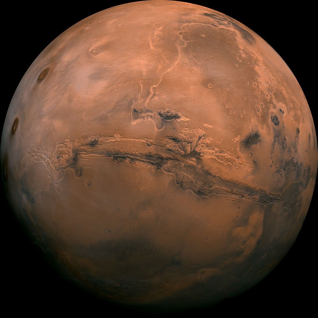
    Featured image: NASA/JPL-Caltech. Mosaic made from 102 Viking Orbiter images. Public-domain NASA imagery; contextual image, not the laboratory experiment or a confirmed habitat. Image source.

  • Ice-Giant Dynamo Models Suggest Magnetic Maps May Change Over Decades

    Ice-Giant Dynamo Models Suggest Magnetic Maps May Change Over Decades

    The magnetic maps of Uranus and Neptune rest on a remarkably small foundation: one spacecraft flyby of each planet. New computer models suggest those maps may also describe fields that change substantially over decades, making their age an important part of how astronomers interpret observations today.

    A study published November 3, 2026, in Communications Physics identifies changing electrical conductivity with depth as a route to producing the ice giants’ unusual magnetic geometry. It does not measure a newly shifted magnetic pole. Instead, it tests a physical mechanism capable of generating fields resembling those Voyager 2 encountered.

    Conductivity changes the dynamo

    Planetary magnetic fields arise from moving, electrically conducting material inside a planet. In the simulations, making conductivity increase toward greater depth helped produce complex fields rather than a dominant magnetic alignment with the rotation axis. The result appeared across different thicknesses of the modeled convecting shell.

    The University of Texas at Austin’s November 3 announcement explains why such a gradient is plausible. Under intense pressure and heat, water-rich material can become increasingly conductive as molecules break into ions. The actual composition and structure of both planetary interiors remain uncertain.

    The contrast with Earth is striking. The university’s summary gives magnetic dipole tilts of about 59 degrees for Uranus and 47 degrees for Neptune, compared with roughly 11 degrees for Earth. Those angles are one description of the difference; the ice giants also have complicated magnetic structures that cannot be captured by a simple tilted bar magnet.

    A prediction that needs a time series

    Some simulated intervals show large changes over decades, while others evolve slowly. The paper therefore treats temporal variation as plausible, with its real extent poorly constrained. A model that reproduces one observed configuration cannot by itself establish how the actual planet traveled to that configuration or where its field points now.

    Researchers are examining infrared auroral observations from Webb for clues. Auroral patterns can help test magnetic geometry, but interpreting them also requires understanding how particles and atmospheric conditions produce the emission. New spacecraft measurements would provide a more direct comparison with Voyager.

    The practical lesson is about time as well as distance. A remote planet’s old measurement remains valuable, but assuming that it is a permanent map can build hidden uncertainty into newer results. These simulations make that assumption testable.

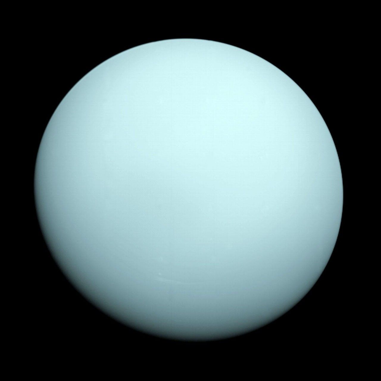
    Featured image: NASA/JPL. Voyager 2 photograph of Uranus, January 14, 1986. Public-domain NASA imagery. Image source.