DARK FIRESORIGINS UNKNOWN

Author: Dark Fires

  • Why Two Aircraft Altitudes Can Disagree Without an Impossible Maneuver

    Why Two Aircraft Altitudes Can Disagree Without an Impossible Maneuver

    Investigation guide · Sources checked November 5, 2026, Chicago time.

    A flight-tracking screenshot can look decisive: an aircraft was at a particular altitude, so it could not have been the light in a witness’s video. Before using that number to exclude a candidate, check what kind of altitude it represents. Two legitimate values can describe the same aircraft without representing the same measurement.

    Pressure altitude is not geometric height

    The FAA’s ADS-B FAQ distinguishes barometric and geometric altitude. The transmitted barometric value is pressure altitude, corresponding to an altimeter set to the standard 29.92 inches of mercury. The geometric value comes from GPS and represents height above the Earth ellipsoid.

    Those are different reference systems. Neither should automatically be read as height above the observer’s roof or nearby terrain. A comparison that silently treats all three as interchangeable can create an apparent discrepancy before any unusual object has entered the analysis.

    Read the actual data field

    The ADS-B Exchange streaming documentation provides a concrete example. It labels alt_baro as barometric altitude in feet and alt_geom as geometric GNSS altitude in feet. It also distinguishes measured altitude from selected autopilot altitude fields. A pilot’s selected level is not proof that the aircraft has reached it.

    The documentation says an unavailable field may be absent, and the barometric field can contain a ground-state indicator rather than a numerical altitude. Missing information should remain missing. Converting an absent value into zero, or interpreting a ground indicator as a measured height, introduces an error of the analyst’s own making.

    A fair comparison

    Our recommended workflow is to preserve the original field name, units, timestamp and provider alongside every extracted value. Record whether the website explains corrections applied to its display. If its treatment is unclear, say so rather than guessing from the map label.

    Next, keep aircraft altitude separate from observer elevation and apparent angle above the horizon. A proper comparison needs a common vertical reference and the aircraft’s position relative to the observer. The existence of a plausible aircraft nearby is a lead, not a completed identification.

    Finally, test the proposed match against the sequence: direction, time, changing position and visibility. If the claimed mismatch survives a documented comparison, retain it as a real limitation. If it disappears after correcting incompatible altitude definitions, explain that transparently.

    The lesson is narrow but important. An altitude disagreement does not prove an exotic maneuver, and an altitude agreement does not prove an aircraft identification. The numbers become evidence only after their definitions are made explicit.


  • Inside the Naval Postgraduate School’s UAP Issue: Measurements Before Conclusions

    Inside the Naval Postgraduate School’s UAP Issue: Measurements Before Conclusions

    Research reading guide · Sources checked November 5, 2026, Chicago time. The journal issue is labeled Spring 2026; this is not a new November release.

    The Naval Postgraduate School’s special UAP edition of Combating Threats Exchange offers a useful alternative to treating every official publication as either disclosure or dismissal. Its central question is methodological: what information would make an unusual observation possible to investigate?

    The guest editors’ letter describes an NPS effort developed in close partnership with the All-domain Anomaly Resolution Office. The stated priorities include scientific methods, less stigma around reporting, and collaboration. Publication by a military institution establishes provenance, not the truth of every interpretation inside it.

    Start with what a sensor actually measures

    One especially useful contribution is former AARO science adviser Randy Bostick’s article on data vetting and accessibility. He distinguishes recorded measurements from conclusions drawn from them. A description of unusual propulsion is already an interpretation, not a direct sensor reading.

    Bostick argues that supporting metadata matters because calculated quantities depend on how observations were collected. Sensor settings, platform location and motion can determine whether another analyst can reproduce a claimed speed or size. His proposal is therefore relevant even when readers disagree with an eventual identification: the intermediate steps should remain inspectable.

    Keep the interview’s date attached

    The issue also contains an interview with AARO director Jon Kosloski conducted December 4, 2025. He describes inadequate data as a major investigative obstacle and explains that military sensors are optimized for particular missions rather than general scientific observation. Those remarks should be attributed to that interview, not presented as a fresh November 2026 statement.

    Kosloski’s account is an institutional perspective. It helps explain AARO’s priorities, but it does not independently settle any individual case or establish that every unresolved report has the same cause.

    A practical way to read it

    The official contents page links separate articles on event-based sensing, Ukrainian observations and practical photography. Readers can inspect these individually rather than relying on a summary of the whole issue.

    For each claimed result, ask three questions: What was measured? Which assumptions turn that measurement into a physical claim? What information would let someone else check it? This is an editorial reading framework, not a finding announced by NPS. It keeps an interesting publication useful without turning institutional interest into evidence of an extraordinary origin.

    Featured photograph: The Pentagon, May 15, 2023. U.S. Air Force Staff Sgt. John Wright / DoD, public domain. Institutional context, not the Naval Postgraduate School campus.

  • NASA’s Ka-Band Awards Target the Hardest Part of a Commercial Relay Transition

    NASA’s Ka-Band Awards Target the Hardest Part of a Commercial Relay Transition

    NASA’s November 4, 2026, selection of three companies for Ka-band relay development addresses a practical problem in space infrastructure: changing the network while keeping existing spacecraft connected. The agency wants services compatible with hardware already in orbit, where replacing a radio is rarely a straightforward option.

    The contract announcement names Astranis Space Technologies, Global Enterprise Solutions and Viasat. Their maximum potential awards, including future options, are $264.3 million, $340.4 million and $460.9 million respectively. Those ceilings should not be confused with money already committed to completed systems. Initial work runs from November 4 to May 3, 2027; optional phases could extend through 2029 and reach an orbital demonstration.

    NASA is seeking complete services encompassing spacecraft, ground equipment, launch, operations and integration. The compatibility requirement distinguishes this effort from developing communications terminals for missions that have not yet launched.

    Keeping older missions in the conversation

    The backdrop is NASA’s planned move away from its government-owned Tracking and Data Relay Satellite system. Its TDRS overview describes satellites distributed over the Atlantic, Pacific and Indian oceans, relaying information between spacecraft and Earth. Users include the International Space Station, Hubble and Earth-observing missions. This is working infrastructure with established customers, rather than an empty market waiting for its first network.

    In its commercial-transition explanation, NASA identified backward compatibility, anomaly support, terminal availability and cost models among the questions needing industry input. That earlier discussion helps explain why a new provider’s headline data rate cannot, by itself, settle the transition.

    What the awards establish

    Our reading is that the difficult engineering boundary lies between an existing mission’s fixed capabilities and a new supplier’s operating system. A service must fit the spacecraft that actually needs it. Successful migration also requires confidence in the complete route from orbital user to ground operations.

    The contracts create a path to test that proposition; they do not establish that replacement services are operational today. The next meaningful milestones will be demonstrated compatibility, risk reduction and decisions on later options. For readers following commercial space, this is a useful reminder that continuity can be as consequential as a brand-new capability.

    For existing missions, preserving a dependable connection is a prerequisite for making any newer network useful.

    Featured image: NASA/Morgan Johnson illustration of relay communications, not a depiction of the newly awarded systems. Image source.

  • Weather Balloons and UAP: Why Surface Wind Is Not Enough

    Weather Balloons and UAP: Why Surface Wind Is Not Enough

    An unfamiliar object appears to move against the breeze felt by an observer. Does that rule out a balloon? Only if that breeze represents the air at the object’s actual height and location. For an elevated object, a surface weather report is a starting point rather than a complete test of wind-driven motion.

    A rising balloon samples changing conditions

    Weather balloons carry instrument packages called radiosondes. The National Weather Service describes an approximate ascent rate of 300 metres per minute and explains that tracking the package provides wind speed and direction aloft. A flight can last more than two hours and travel hundreds of kilometres from its launch point. Those figures describe typical sounding operations, not a fixed trajectory for every balloon. See the NWS radiosonde factsheet.

    As a balloon rises, it encounters successive layers of air. Wind speed and direction can differ between those layers, so its horizontal track can curve without powered steering. NOAA’s radar-velocity guide illustrates winds changing direction with height and identifies that change as wind shear. A surface flag cannot reveal the entire profile above it.

    Ascent adds another ingredient. Even in weak horizontal wind, a buoyant balloon can gain height. Its vertical motion should not be judged as though it were simply a leaf carried horizontally past a weather station. Conversely, knowing that balloons rise does not establish that any particular rising light or shape is a balloon.

    A simple trajectory example

    Suppose, for illustration, a balloon rises steadily at 300 metres per minute. It would gain about 3 kilometres in ten minutes. If its horizontal drift averaged 15 metres per second over those ten minutes, it would also move about 9 kilometres horizontally: 15 × 600 = 9,000 metres. Those speeds and the constant-ascent assumption are chosen for arithmetic, not reconstructed from an incident.

    If the wind changes direction halfway through the climb, applying one wind vector to the whole interval gives the wrong endpoint. A more useful calculation divides the ascent into shorter periods, applies a wind estimate appropriate to each height and time, and adds the resulting displacements. Uncertainty in launch position, ascent rate and winds should produce a range of possible tracks rather than a single apparently exact line.

    Test the balloon hypothesis with the right records

    Start with the sighting’s time, observer location, viewing direction and any supported altitude estimate. Then seek nearby upper-air observations and candidate launch records. NOAA’s Integrated Global Radiosonde Archive includes wind direction, wind speed, height information and elapsed time since launch. Its documentation also warns that vertical and temporal resolution vary.

    A sounding is not a simultaneous measurement of every point overhead. The instrument moves while it climbs, and a nearby station may sample a different air mass or time. Model wind profiles can help fill gaps, but they remain estimates. Comparing several plausible heights is especially important when the object’s altitude is unknown.

    A credible match joins the launch time and location to a plausible trajectory, then checks whether that trajectory agrees with the observed direction and timing. Agreement with winds supports a balloon explanation but does not uniquely identify the object. A mismatch with ground-level wind alone is weak grounds for rejecting it. The useful question is whether the full set of observations fits a realistic flight through the atmosphere.

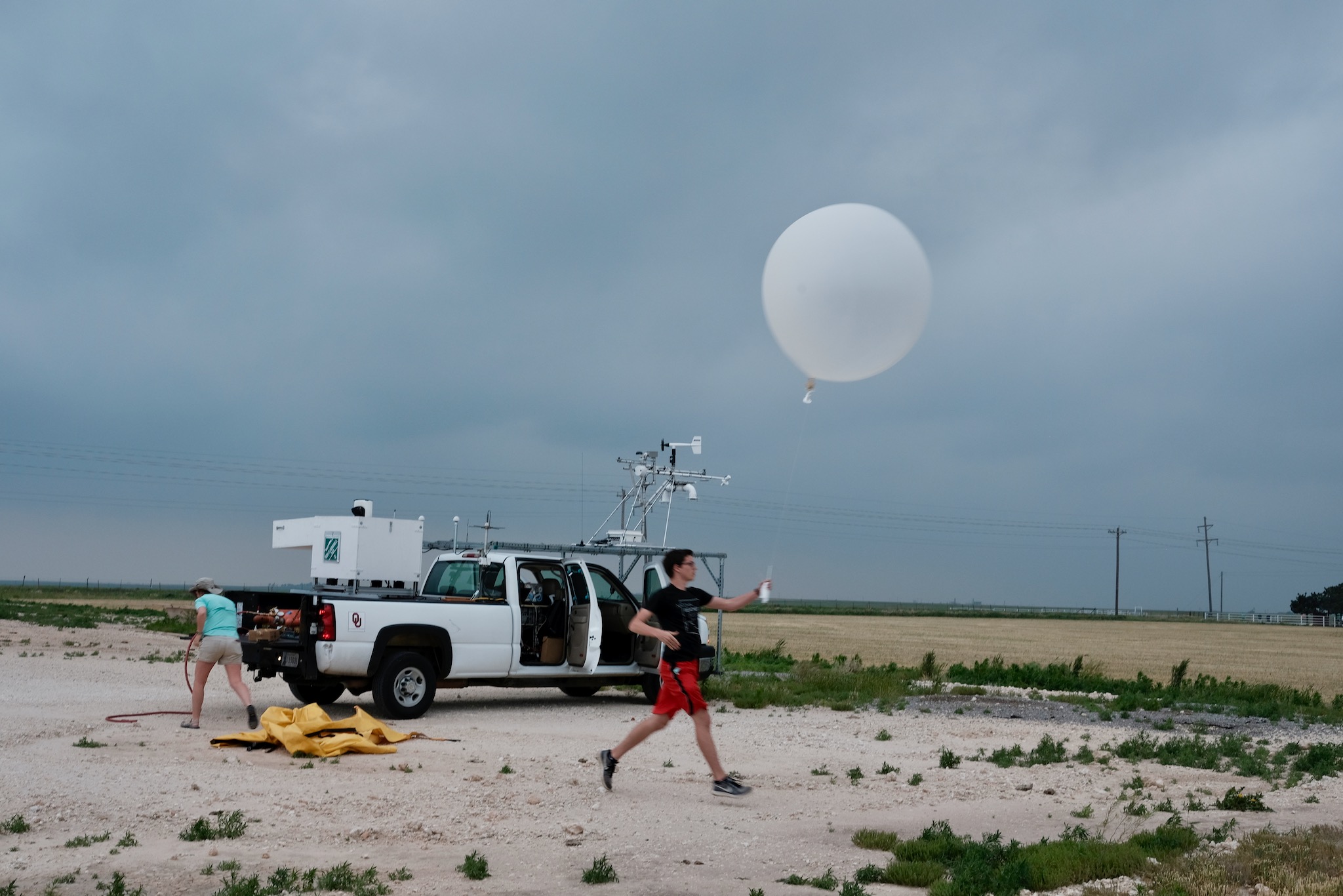
    Featured image: OU CIMMS researcher Nolan Meister releases a weather balloon carrying upper-air instruments on May 23, 2019. Context photograph, not a UAP sighting. Photo: Mike Coniglio / NOAA NSSL, public domain.

  • NASA Details Drone Test of a System That Can Choose Safer Planetary Landing Sites

    NASA Details Drone Test of a System That Can Choose Safer Planetary Landing Sites

    A drone flight over California’s Rogers Dry Lake is helping NASA prepare spacecraft to choose safer landing spots on other worlds. In a report published November 4, the agency described a successful demonstration of SPLICE, a guidance, navigation and control system designed for precise planetary landings.

    The flight took place on August 27, not on the publication date. An Alta-X drone carried the experiment through simulated lunar descent and landing maneuvers near NASA’s Armstrong Flight Research Center in Edwards, California. NASA had previously shared an image of that flight; the new account adds detail about the integration work and the next stage of testing.

    Choosing a place to touch down

    SPLICE stands for Safe and Precise Landing–Integrated Capabilities Evolution. During the drone experiment, its guidance system mapped the terrain and assessed possible landing areas. The system is designed to redirect a vehicle if its original target proves unsafe. High-resolution elevation maps turn sensor measurements into a representation of the ground that the navigation software can evaluate.

    Researchers at Johnson Space Center developed the payload, while Armstrong specialists helped integrate it with the drone. Tests in June and July checked communications, data handling, telemetry and command-and-control performance. NASA says that work prepared the team for a full-scale test at Voyager Technologies in Mojave, California, planned for later in November.

    Several tools work together

    The broader SPLICE architecture combines sensors, software and computing rather than relying on one measurement. Terrain-relative navigation compares live camera images with previously collected orbital imagery to establish where a spacecraft is. Navigation Doppler lidar uses returning laser signals to estimate altitude and velocity.

    A separate hazard-detection lidar builds a three-dimensional view of the landing field. Software examines that terrain for hazards such as rocks and steep slopes, while the descent-and-landing computer processes the information and supports selection of a safer site. Guidance then has to translate that selection into a trajectory the vehicle can actually fly.

    These jobs address different questions: where the vehicle is, how it is moving, what lies below, and how to reach an acceptable touchdown point. Integrating the answers is essential when the surface is approaching and a late change must remain within the vehicle’s capabilities.

    A terrestrial test with a planetary purpose

    NASA’s earlier flight-image release described the technology’s intended application to the Moon, Mars, icy worlds and other destinations. Reaching scientifically valuable terrain can require navigating near features that make a landing difficult. Better onboard assessment could help missions approach those locations more precisely.

    The California demonstration is a development milestone, not proof that the complete system has performed a lunar landing. A drone over a dry lake does not reproduce every condition a planetary lander will face. Its value is in exercising the connected navigation and guidance functions on a moving vehicle before more demanding tests.

    The next reported step is the planned full-scale Mojave test. For now, the August flight gives engineers evidence that the payload and flight platform can work together while carrying out a simulated descent.

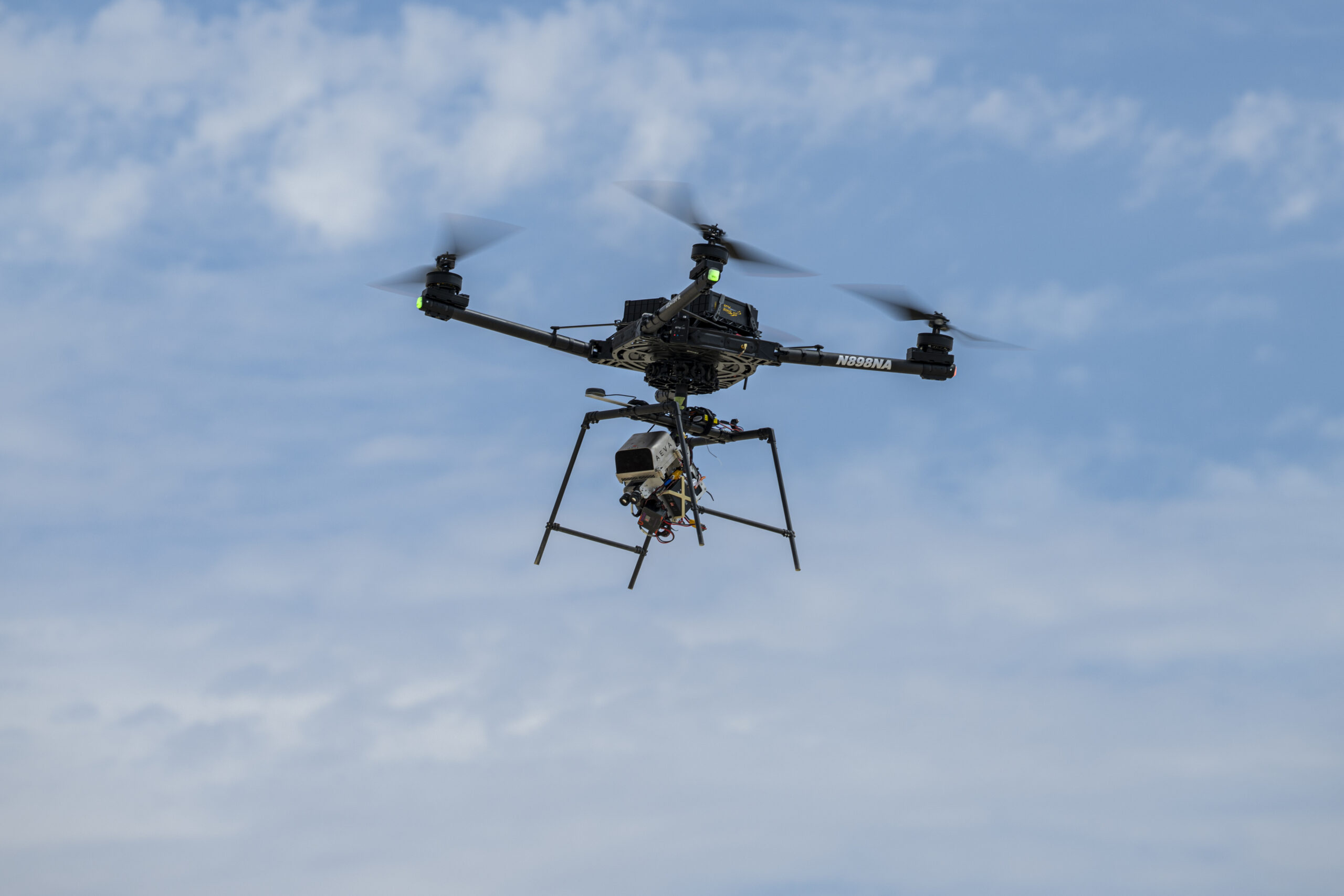
    Featured image: An Alta-X drone flies the SPLICE experiment near NASA Armstrong on August 27, 2026. Credit: NASA/Ryan Kline. Image licence.

  • MetOp-SG-B1 Leaves Storage as Engineers Prepare Weather Satellite for Launch

    MetOp-SG-B1 Leaves Storage as Engineers Prepare Weather Satellite for Launch

    Europe’s next MetOp weather satellite has moved from protected storage into the cleanroom phase of its launch campaign. In a November 4 update, the European Space Agency said MetOp-SG-B1 had been removed from its transport container at Europe’s Spaceport in French Guiana. Engineers are preparing to reactivate it ahead of a launch planned toward the end of 2026.

    The spacecraft reached Kourou on October 16 after leaving Bordeaux aboard the sail-assisted vessel Canopée on October 6. Its container maintained a dry, nitrogen-rich environment at a steady 22 degrees Celsius during storage.

    Switching on the satellite, carrying out final checks and fuelling it are still ahead in the reported sequence. It will then be enclosed in its Ariane 6 rocket’s protective fairing and moved to the launch pad. ESA has not announced an exact launch date in this update.

    One half of a complementary pair

    MetOp-SG-B1 is part of a weather-observing system built around two different satellite types. The A and B spacecraft carry complementary instruments, allowing their measurements to be combined rather than simply duplicating the same observations. MetOp-SG-A1 launched on August 13, 2025.

    According to ESA’s mission overview, the full programme consists of six spacecraft arranged as three successive pairs. They will operate in polar orbit at approximately 800 kilometres altitude, providing global observations for weather forecasting and climate work over more than two decades. Temperature, precipitation, clouds and winds are among the variables the system is designed to measure.

    The successive-pair approach makes continuity part of the mission design. A forecasting system needs repeated measurements, while climate research also depends on observations sustained over long periods. The programme is intended to serve both timescales.

    What the B satellite adds

    ESA’s instrument description lists five payloads for the B-type spacecraft. A scatterometer measures ocean-surface winds and land-surface soil moisture. A radio-occultation sounder supplies atmospheric temperature and humidity profiles, along with information about the ionosphere.

    The microwave imager will observe precipitation and sea-ice extent, while the ice-cloud imager measures ice within clouds. The Argos-4 data-collection system gathers and relays measurements from platforms such as buoys, ships, balloons and aircraft.

    This mix connects observations made from orbit with information collected closer to the surface. It also illustrates why a weather satellite is more than a camera looking down at cloud tops: different instruments reveal different physical properties of the atmosphere, oceans and land.

    Preparation, not yet liftoff

    The current milestone moves the spacecraft closer to flight, but important work remains between removal from storage and launch. The distinction matters when reading an announcement about waking a satellite: preparation for switch-on is not confirmation that activation or final testing has finished.

    For MetOp-SG-B1, the next checkpoints are those campaign operations. Once they are completed, the spacecraft can proceed toward joining the A1 satellite and expanding the measurements available to forecasters.

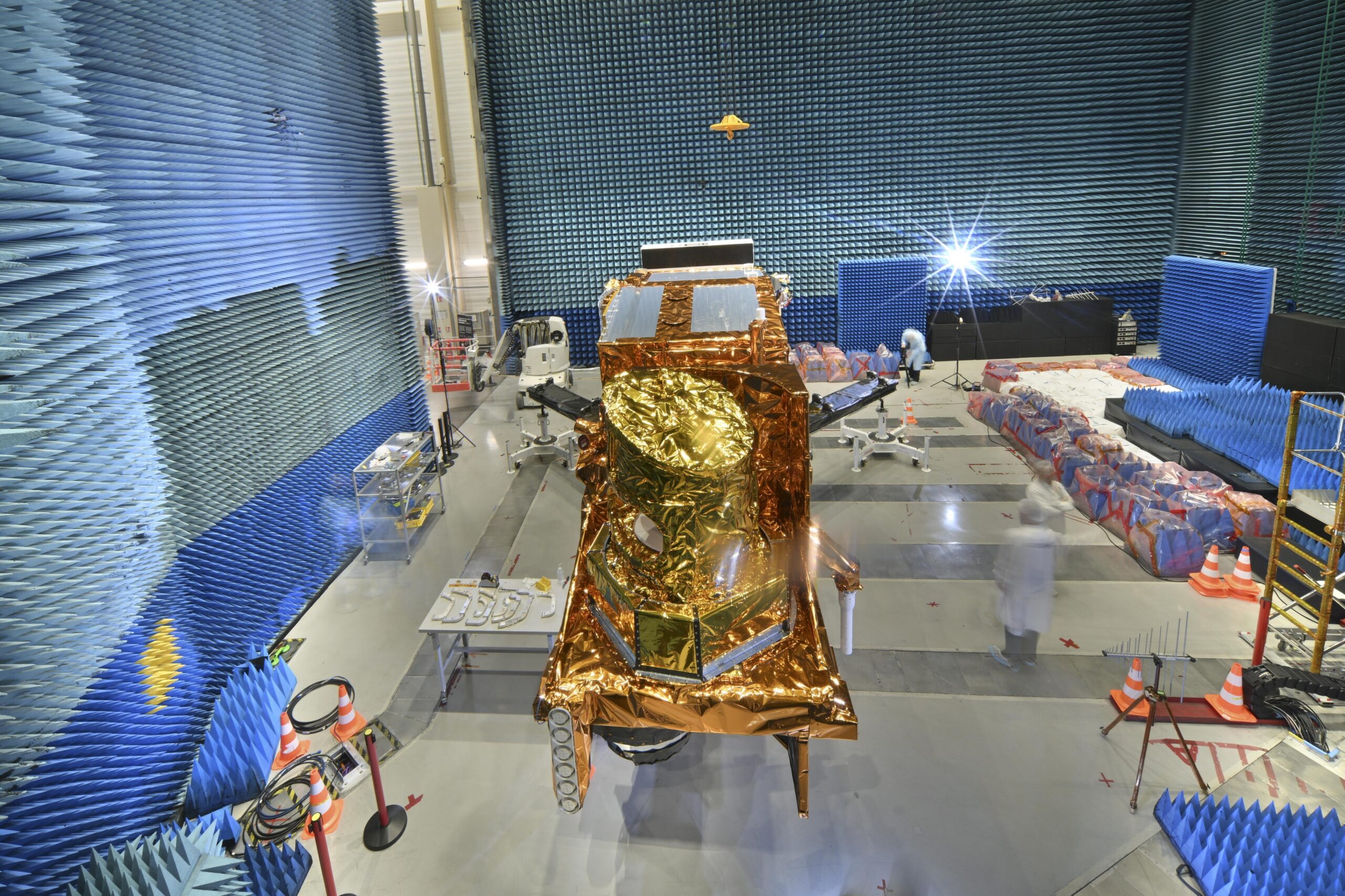
    Featured image: MetOp-SG-B1 during earlier testing in Toulouse, in an image published November 24, 2025. Credit: ESA–M. Pédoussaut, CC BY-SA 3.0 IGO. Displayed crop. Image licence.

  • Swift Re-Entry Confirmed Over North Sumatra After Nearly 22 Years in Orbit

    Swift Re-Entry Confirmed Over North Sumatra After Nearly 22 Years in Orbit

    NASA’s Neil Gehrels Swift Observatory re-entered Earth’s atmosphere on November 4, closing the spacecraft’s nearly 22-year stay in orbit. The U.S. Space Force confirmed re-entry at 7:39 a.m. Eastern Standard Time, or 6:39 a.m. in Chicago, according to NASA’s updated mission notice.

    The reported location was over Indonesia’s North Sumatra region, near 3.4 degrees north latitude and 98.6 degrees east longitude. NASA said it expected most of the spacecraft to burn up during atmospheric passage, although some components may have survived. The notice does not identify recovered debris or provide a confirmed ground-impact location.

    A confirmed end to the orbit

    The new development is the confirmation of re-entry itself. Swift’s science shutdown had already been announced in October. NASA originally published its latest notice on November 2, then revised it on November 4 after receiving the Space Force confirmation. Readers following the earlier forecast can therefore distinguish the predicted return from the now-confirmed event.

    The coordinates describe the reported re-entry location. They should not be treated as a precise address for surviving hardware. Likewise, the possibility that components survived is not evidence that fragments have been found. NASA’s short update leaves those questions open.

    Why Swift mattered to a changing sky

    Swift launched on November 20, 2004, with a two-year primary mission. Its specialty was speed: it could catch a brief high-energy flash and turn toward it while the aftermath was still bright. That ability made the observatory particularly valuable for gamma-ray bursts, events associated with catastrophic stellar deaths and mergers involving compact objects.

    NASA’s spacecraft description explains how its three instruments divided that work. The Burst Alert Telescope detected and located a burst, while the X-Ray Telescope and Ultraviolet/Optical Telescope examined its afterglow. After a detection, Swift could autonomously repoint in roughly 20 to 100 seconds. Observations across different wavelengths gave researchers a more complete view of an explosion than a single instrument could provide.

    Its alerts also helped other observatories turn toward the same source. That coordination mattered because a transient can change substantially while astronomers are still organizing a follow-up. Swift made the initial discovery and the subsequent observations parts of a connected process.

    The spacecraft is gone; its observations remain

    Over time, Swift became a broader astronomical observatory. Its work extended to stellar flares, supernovae, active galaxies and stars disrupted by massive black holes, as well as comets and asteroids closer to home. NASA’s mission page preserves access to that scientific record and the observatory’s history.

    November 4 marks a physical endpoint for the satellite, rather than a new explanation for its earlier shutdown. The immediate news is now settled: Swift has returned to the atmosphere. Its contribution to astronomy continues through the measurements and coordinated observations accumulated during more than two decades of operation.

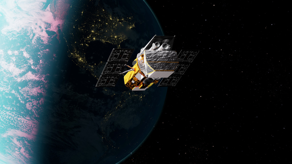
    Featured image: Artist’s concept of Swift in orbit, not an image of its November 4 re-entry. Credit: NASA’s Goddard Space Flight Center Conceptual Image Lab. Image licence.

  • Radar Doppler and UAP: What Radial Velocity Actually Measures

    Radar Doppler and UAP: What Radial Velocity Actually Measures

    A radar report that gives an unexplained object’s speed invites a basic question: speed in which direction? A Doppler measurement describes motion along the radar’s line of sight. Turning that number into a complete flight path requires additional information. The distinction matters when assessing claims of hovering, sudden acceleration or extraordinary performance.

    The component the radar measures

    For a stationary radar observing an isolated target, radial velocity is the rate at which the distance between them changes. Motion directly toward or away from the antenna contributes fully. Motion across the line of sight contributes only partly, and motion exactly perpendicular to it contributes nothing at that instant. NOAA’s explanation of radar velocity sets out these geometric limits.

    A useful expression is vr = v cos θ, where v is the target’s speed relative to the radar and θ is the angle between its velocity and the outward line of sight. Taking outward motion as positive makes approaching motion negative. The angle is three-dimensional: horizontal bearing alone is insufficient when vertical motion matters.

    Consider an illustrative target moving at 100 metres per second, with its velocity 60 degrees from the outward radar line. Its radial velocity is 100 × cos 60° = 50 metres per second. At 90 degrees, the instantaneous radial velocity would be zero even though the target still moves at 100 metres per second. These are calculated examples, not measurements from a UAP encounter.

    A single number leaves many possibilities

    A reliable, unambiguous radial speed supplies a lower bound on the magnitude of relative velocity. It supplies no upper bound by itself: different transverse components can accompany the same radial component. Dividing by an assumed cosine does not recover a measured total speed. Near 90 degrees, a small error in the assumed angle can produce a very large error in that calculation.

    Zero radial velocity also does not establish a sustained hover. A target passing across the radar’s view can momentarily have zero range rate at its closest approach. As the viewing direction changes, the radial component can change even if the target maintains a straight path and constant speed. A changing Doppler value therefore needs geometric interpretation before it becomes a claim of acceleration.

    Check ambiguity and the reported product

    Pulse-Doppler measurements have sampling limits. Velocities outside the unambiguous interval can fold into it, potentially reversing the displayed sign. A 1995 Navy weather-radar training manual hosted by the National Weather Service explains velocity aliasing and warns that correction algorithms can occasionally produce incorrectly dealiased data. A colour transition or isolated extreme value should be checked against the instrument’s operating mode and processing history.

    NOAA’s glossary defines mean Doppler velocity as a reflectivity-weighted average of target velocities within a pulse-resolution volume, measured toward or away from the antenna. That is different from a confirmed track of one solid object. Equally, a tracking radar may derive a velocity vector from successive position measurements or combine multiple sensors. Calling every reported radar speed “only Doppler” would discard information those systems may actually provide.

    For a defensible UAP assessment, ask what product is being quoted, whether the radar platform was moving, how platform motion was handled, whether aliasing was resolved, and what independent range and angular measurements exist. Preserve those distinctions in the conclusion. Radar can constrain motion powerfully, but the strength of a three-dimensional speed claim depends on the measurements used to reconstruct it.

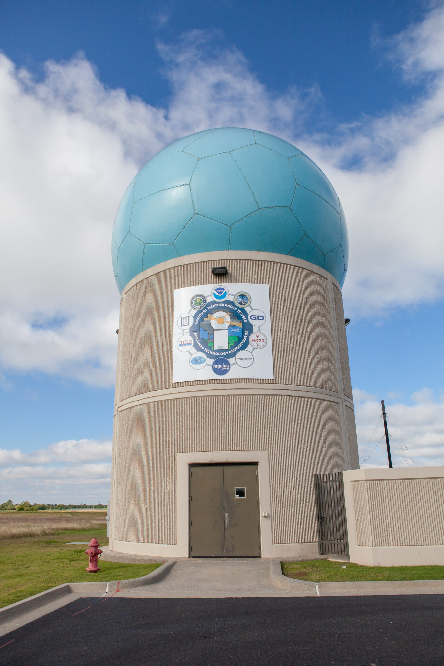
    Featured image: The Advanced Technology Demonstrator radar at NOAA’s National Severe Storms Laboratory. Context photograph, not imagery of a UAP incident. Photo: NOAA/NSSL, public domain.

  • Video Compression and UAP: Why the Camera File Matters

    Video Compression and UAP: Why the Camera File Matters

    A distant light appears to split, acquire a dark outline or change shape in a short sky video. Before treating those pixels as features of an unidentified object, establish which version of the recording they came from. The camera file, an exported edit and a social-media copy can contain different visual information.

    What compression can change

    Lossy compression reduces the amount of information needed to store and transmit a recording by discarding some data. Adobe’s encoding documentation distinguishes compression within an individual frame from temporal compression, which exploits relationships between frames. A decoded video frame is therefore not necessarily an independently stored photograph.

    Compression and resizing are separate operations, and both can affect the result. Apple’s video-quality engineering presentation demonstrates blockiness, blur and disappearing detail introduced by encoding and downscaling. When a target occupies only a small area, a modest change at its boundary can become a large fraction of its apparent shape.

    The practical consequence is narrow but important: a jagged edge or small appendage in a compressed copy needs verification before it becomes a claim about structure. Seeing an artifact-like pattern does not establish that the entire light is an artifact.

    Compare versions rather than enlargements

    Request the file directly exported or copied from the recording device, rather than a screen recording of a player. Ask whether it has been trimmed, stabilized, resized, enhanced or sent through a messaging service. Call it the camera file only when that description is supported. A download labeled “original” by a website may simply be the earliest upload available there.

    The camera file may already use lossy compression. Its value is that it avoids additional, undocumented transformations. Adobe’s compression guidance warns that repeatedly re-encoding compressed material can further degrade quality.

    Compare matching moments in the earliest available file and the circulated copy. Keep the surrounding scene visible, then inspect equivalent crops with the enlargement method recorded. Enlarging an image makes existing samples easier to see; it does not supply the measurements that were discarded. Smooth-looking enlargement should not be mistaken for newly resolved detail.

    Check whether a disputed feature survives in the earlier version, across neighboring frames and under more than one straightforward display method. If it appears only after a particular export, that is evidence about the export’s effect. If it is present in the camera file, further questions about the optics, sensor and scene remain.

    Match the conclusion to the test

    A useful comparison can be simple: “The narrow projection is visible in the repost but is not resolved in the camera file.” That statement identifies the observation and its limit. “Compression proves the object was fake” goes beyond the comparison.

    A technical analyst can also make a documented test export from the source and see whether a similar distortion appears. Matching an artifact strengthens a proposed mechanism, but unknown platform settings may prevent exact reproduction. Keep the test copy separate and disclose its settings.

    When only a small, heavily processed clip survives, some shape questions may be unanswerable. The right response is to reduce the precision of the claim. A recording can still establish that a light was present while being inadequate to establish its outline, construction or a momentary physical transformation.

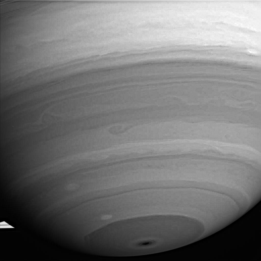
    Featured image: Cassini’s July 31, 2005 infrared view of Saturn retains block-shaped compression artifacts after enhancement. It illustrates a documented imaging limitation, not a UAP observation. Credit: NASA/JPL/Space Science Institute. Image licence.

  • Lens Flare in UAP Videos: How to Test a Ghost Image

    Lens Flare in UAP Videos: How to Test a Ghost Image

    A small light that darts across a sky video may be an object in the scene, or a reflection created inside the camera. Telling those possibilities apart requires more than recognizing a familiar green dot. A useful lens-flare test asks whether the light’s position follows the camera’s optical geometry throughout the recording.

    How a camera creates an extra light

    Light does not pass perfectly through every glass surface. Some reflects, and a fraction can reach the sensor after bouncing within the optical system. Canon’s explanation of lens coatings describes how these reflections create displaced ghost images and flare. Coatings reduce the problem; their presence does not make every photograph immune.

    A distinct ghost and a broad wash of glare are different appearances of unwanted light. Neither has to resemble the source that produced it. A bright lamp can therefore generate a faint feature elsewhere in the frame without a second lamp being present at that location.

    Test a relationship across frames

    The peer-reviewed paper Geometry by Deflaring derives a useful constraint for aligned, radially symmetric optical systems: aperture ghosts concentrate around a line connecting the bright source’s image and the point where the optical axis meets the image plane. Camera movement changes that relationship in a predictable geometric way.

    The paper also documents a weak ghost away from the predicted line. Its model permits the illuminating source to be outside the frame. These qualifications matter when testing a real recording.

    Examine several well-separated, uncropped frames. Mark the suspected ghost and plausible bright sources. Ask whether source-to-ghost lines pass near a consistent optical center as the camera changes direction. Include intervals when the proposed relationship fits poorly.

    The center of a reposted rectangle need not be the optical center. Cropping and stabilization can complicate that reference. If the processing history is unknown, disclose the limitation rather than forcing a precise fit.

    Separate camera behavior from scene behavior

    Compare the light with background landmarks too. Camera shake moves genuine scene features as well as ghosts. A repeatable relationship to the source and optical geometry is a more useful test.

    Where the equipment is available, a controlled recording of an ordinary bright lamp with the same camera, lens and accessories can test whether a similar ghost appears. Record the setup and preserve unsuccessful comparisons. A resemblance becomes more useful when it includes movement and position, rather than color alone.

    Do not reject an optical explanation solely because the bright source disappears at the frame edge. NASA’s STEREO reflection examples show Venus producing reflections even after leaving the camera’s field of view. They also show that internal reflections can grow into large, unfamiliar shapes.

    A successful test supports a specific explanation for a specific feature. It does not identify every other feature in the recording or discredit the witness. If there is no original framing, no plausible light source and too little camera movement, the honest result may be that the optical hypothesis remains untested.

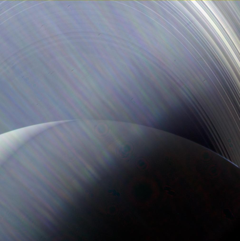
    Featured image: Saturn and its rings photographed by Cassini on June 23, 2013, through sunlight glare in the camera optics. This is an example of an imaging effect, not a UAP photograph. Credit: NASA/JPL-Caltech/Space Science Institute. Image licence.