DARK FIRESORIGINS UNKNOWN

Author: Dark Fires

  • Roman’s First Images Get a December 7 Public Reveal Date

    Roman’s First Images Get a December 7 Public Reveal Date

    NASA will unveil the Nancy Grace Roman Space Telescope’s first images on December 7, 2026, at 3:30 p.m. Eastern, or 2:30 p.m. Central, during an event at the American Geophysical Union meeting in San Francisco.

    The event will stream publicly, and the images will appear online at the same time. NASA’s November 17 advisory follows Roman’s August 30 launch and commissioning journey toward the Sun–Earth L2 region.

    A date to watch, not a result to assume

    Roman’s broad infrared field is designed for surveys addressing dark energy, dark matter and exoplanets. The announcement sets a viewing date, not a scientific result: the images and any findings are still to come.

    Readers can follow the public broadcast through NASA Live. The agency says its first-image release will be posted simultaneously online, so the public need not register as media to see the unveiling.

    Primary source: NASA’s November 17 first-images advisory.

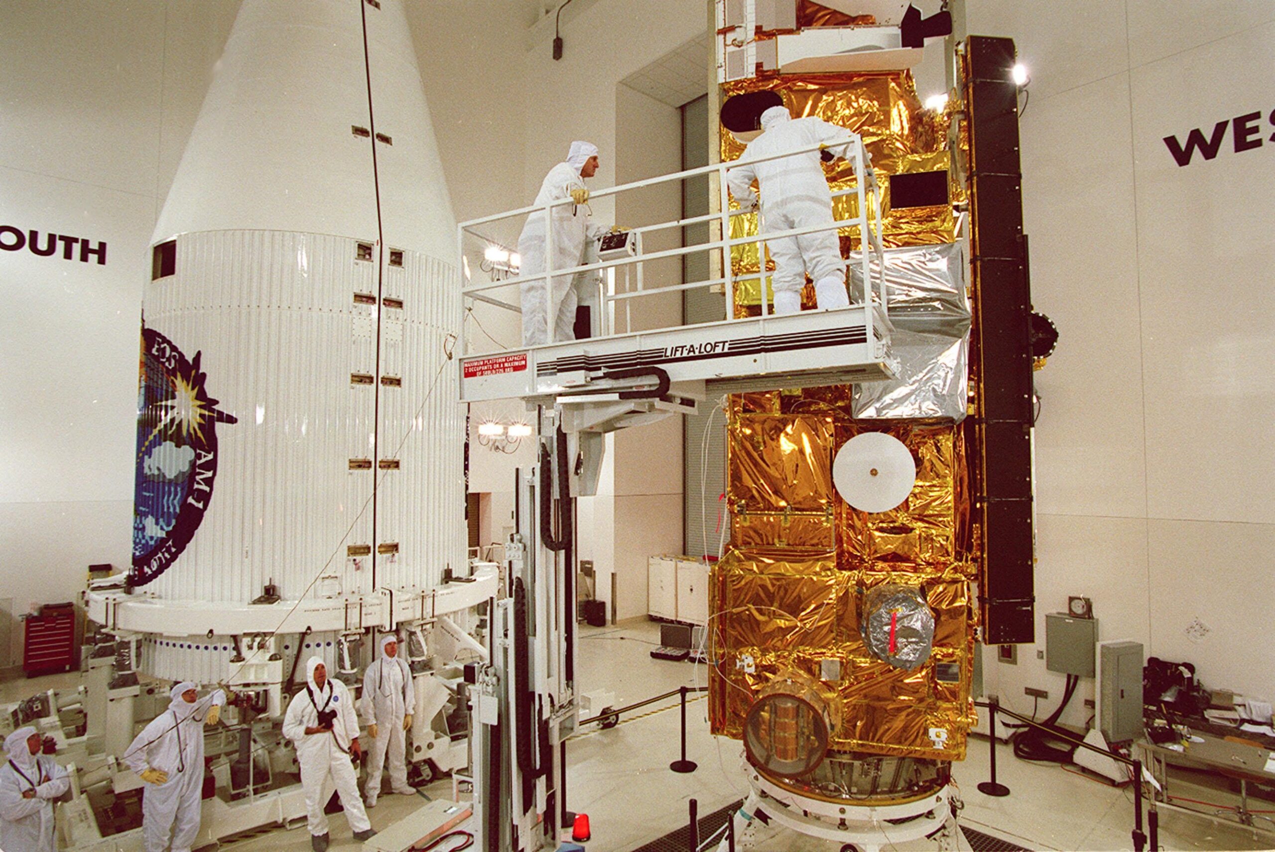
    Featured photograph: Roman in the Goddard clean room on November 25, 2025. Credit: NASA/Jolearra Tshiteya.

  • Lunokhod 1 at 56: The Lunar Rover Whose Tracks Still Tell Its Story

    Lunokhod 1 at 56: The Lunar Rover Whose Tracks Still Tell Its Story

    Luna 17 landed in Mare Imbrium on November 17, 1970, carrying the first successful robotic lunar rover. Over the following ten months, Earth-based operators drove Lunokhod 1 more than 10 kilometers.

    Its eight wheels crossed terrain while instruments examined the soil and cameras recorded the surroundings. Solar power supported daytime work; a radioisotope heater protected the rover through cold lunar nights.

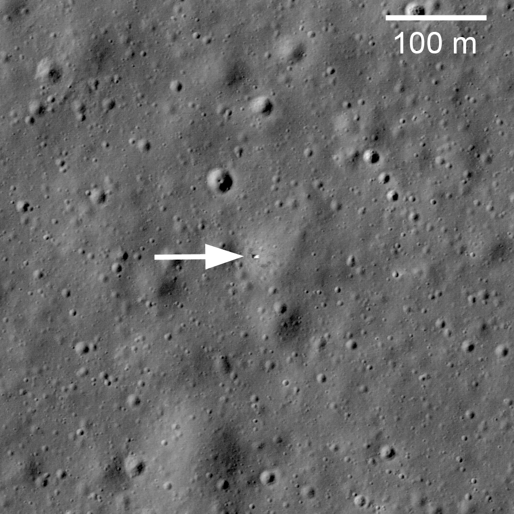
    Decades later, NASA’s Lunar Reconnaissance Orbiter Camera imaged the landing platform, rover and tracks. Those images connect a mission history to hardware still on the surface. The anniversary is a look back, not a newly discovered rover: the cited LROC release dates to March 17, 2010.

    Source: LROC imaging team: Soviet Union Lunar Rovers.

    Featured image: Luna 17 lander and Lunokhod 1 tracks in LROC image M114185541RE. Credit: NASA/GSFC/Arizona State University.

  • NICER’s Science Mission Ends After a Motor-Failure Investigation

    NICER’s Science Mission Ends After a Motor-Failure Investigation

    NASA announced November 17, 2026, that NICER’s science mission has ended. The station-mounted X-ray telescope lost much of its sideways pointing motion in June 2025, forcing observations to pause.

    Robotic inspection ruled out an external obstruction. After investigating, engineers think an internal motor failed. This is a different problem from the sunlight leak patched during a January 2025 spacewalk.

    Eight years of observations remain

    Launched in 2017 for an initial 18-month mission, NICER supplied eight years of observations, including neutron-star measurements and a demonstration of pulsar-based navigation. NASA is completing its public archive and preparing decommissioning and eventual removal from the International Space Station. No removal date was announced.

    The November decision closes the question of returning to science operations after the prolonged pause. It does not erase the measurements already collected.

    Primary source: NASA’s NICER status updates, November 17 announcement and earlier repair history.

    Featured photograph: NICER reflected in Nick Hague’s visor during the January 16, 2025 spacewalk. Credit: NASA/Nick Hague.

  • Terra’s Science Record Will Close December 1, but Its Archive Stays Open

    Terra’s Science Record Will Close December 1, but Its Archive Stays Open

    NASA says Terra will stop collecting science data on December 1, 2026, ending a 27-year mission originally designed for six. Aging hardware and an increasingly unsuitable orbit underpin the decision announced November 17.

    The satellite’s remaining fuel will be used to lower its orbit before final power-off in January 2027. That is a decommissioning plan, not an announced reentry date.

    A long record, not a disappearing archive

    Terra’s five instruments documented changing land cover, atmospheric pollution, fires and ice. Some instrument operations had already ended to conserve power. The retirement closes a stream of new observations, but NASA says the mission’s archive will remain freely available.

    That distinction matters when reading an end-of-mission announcement: the spacecraft can stop taking measurements while its accumulated observations remain available for comparison and further research.

    Primary source: NASA’s November 17 Terra mission update.

    Featured photograph: Workers prepare Terra for encapsulation before its December 1999 launch. Credit: NASA.

  • Before Measuring a UAP Track, Calibrate the Lens

    Before Measuring a UAP Track, Calibrate the Lens

    A curved path across a video frame is not automatically a curved path through space. Lens distortion changes the mapping between scene directions and image pixels. Motion measurements need that mapping, not just a line drawn through visible positions.

    Two kinds of geometric distortion

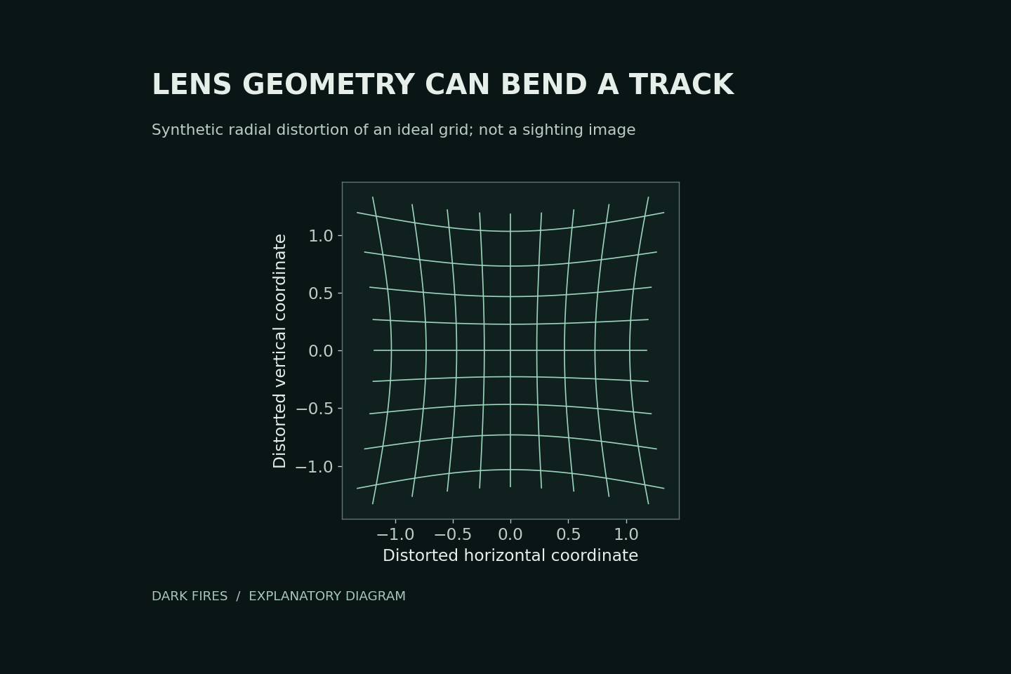
    OpenCV’s camera-calibration documentation distinguishes radial distortion, which can bend straight lines, from tangential distortion associated with imperfect alignment. Radial effects commonly become more noticeable toward an image’s edges.

    Our diagram applies a hypothetical radial mapping to a square grid. It illustrates geometric displacement only. It is not a UAP photograph and does not show how much distortion any particular camera has.

    Measure the camera, not the desired answer

    Calibration uses observations of a known pattern to estimate camera parameters and distortion coefficients. OpenCV’s example uses multiple views of a calibration target, then applies the estimated correction to images.

    For a sighting analysis, retain the unmodified recording and document which camera configuration the calibration represents. Do not tune a correction until the unexplained track becomes straight: that would build the desired conclusion into the measurement.

    Compare corrected and uncorrected positions, report calibration residuals, and propagate remaining position uncertainty into any velocity estimate. Even a well-calibrated pixel trajectory still needs distance and viewing geometry before it yields a physical speed.

    Lens calibration addresses image geometry. It does not by itself correct camera movement, identify the object or prove that an apparent maneuver was an artifact.

    Primary technical source: OpenCV camera calibration tutorial.

    Generated illustration. Original Dark Fires schematic of hypothetical radial distortion, not recorded evidence.

  • A Small P-Value Does Not Identify a UAP’s Cause

    A Small P-Value Does Not Identify a UAP’s Cause

    A statistical result can challenge a model without identifying what produced the observation. That distinction matters when an unusual UAP measurement is described as “too unlikely to be chance.”

    Which probability is being calculated?

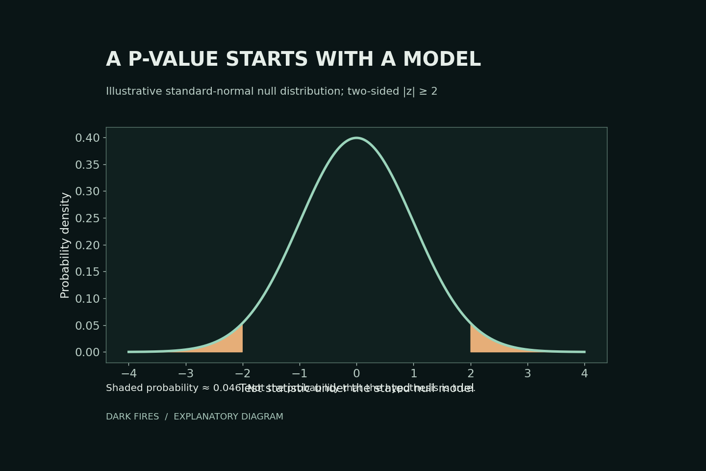
    A p-value describes how incompatible the data are with a specified statistical model, through the probability of a result at least as extreme as the observed test statistic under that model. It is not the probability that the model is true, or that the observation has an extraterrestrial cause.

    Our diagram uses a standard normal model. A two-sided test with a statistic of 2 has a p-value of approximately 0.046: the shaded tails beyond −2 and +2. This does not mean there is a 4.6% probability that the null hypothesis is correct.

    Ask what was left outside the model

    The American Statistical Association’s 2016 statement warns against treating a threshold as a substitute for scientific reasoning. Statistical significance also does not measure the size or importance of an effect.

    In a UAP analysis, inspect calibration errors, the selected sample, model assumptions and the actual magnitude of the discrepancy. Rejecting one ordinary explanation does not test every other ordinary explanation. Compare explicit alternatives and seek independent measurements before turning model disagreement into a claim about origin.

    Primary source: American Statistical Association statement, March 7, 2016.

    Generated illustration. Original Dark Fires plot of a hypothetical normal-model test, not a UAP measurement.

  • UAP Detector Alerts and the Base-Rate Problem

    UAP Detector Alerts and the Base-Rate Problem

    A detector that recognizes most examples of a rare class can still produce many false alerts. Its sensitivity answers one question: how often does it flag a genuine example? An investigator usually needs the reverse: among the alerts, how many are genuine?

    Count the ordinary events too

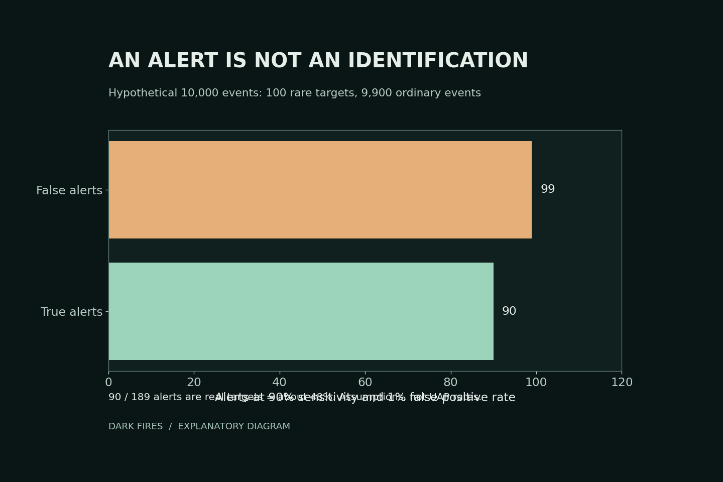
    Consider 10,000 hypothetical events: 100 belong to a target class and 9,900 do not. A detector with 90% sensitivity flags 90 target events. A 1% false-positive rate also flags 99 ordinary events. Only 90 of the 189 alerts, about 48%, belong to the target class.

    These invented numbers do not estimate alien activity, unidentified objects or the performance of any actual UAP system. They demonstrate why the prevalence of the target class matters.

    What Bayes’ theorem changes

    UCAR’s probability documentation explains how Bayes’ theorem combines a prior probability with the likelihood of an observation. Reversing a conditional probability requires that additional information; the detector’s sensitivity alone is insufficient.

    For a real monitoring program, report performance against known examples and ordinary controls, explain how the sample was selected, and show how conclusions change across plausible prevalence assumptions. An unknown base rate should remain an uncertainty, not be replaced with a convenient number.

    Finally, define the target class. An alert for “unusual image” is not a validated detector for “extraterrestrial craft.” Good arithmetic cannot repair an unsupported change in what the classification means.

    Primary technical source: UCAR on conditional probability and Bayes’ theorem.

    Generated illustration. Original Dark Fires chart of the hypothetical example above, not observational UAP statistics.

  • Searching Many UAP Signals Changes the False-Alarm Question

    Searching Many UAP Signals Changes the False-Alarm Question

    A search through many frequencies, time windows or image regions has more opportunities to find a striking coincidence than one preselected test. Reporting only the strongest result hides that difference.

    Twenty chances are not one chance

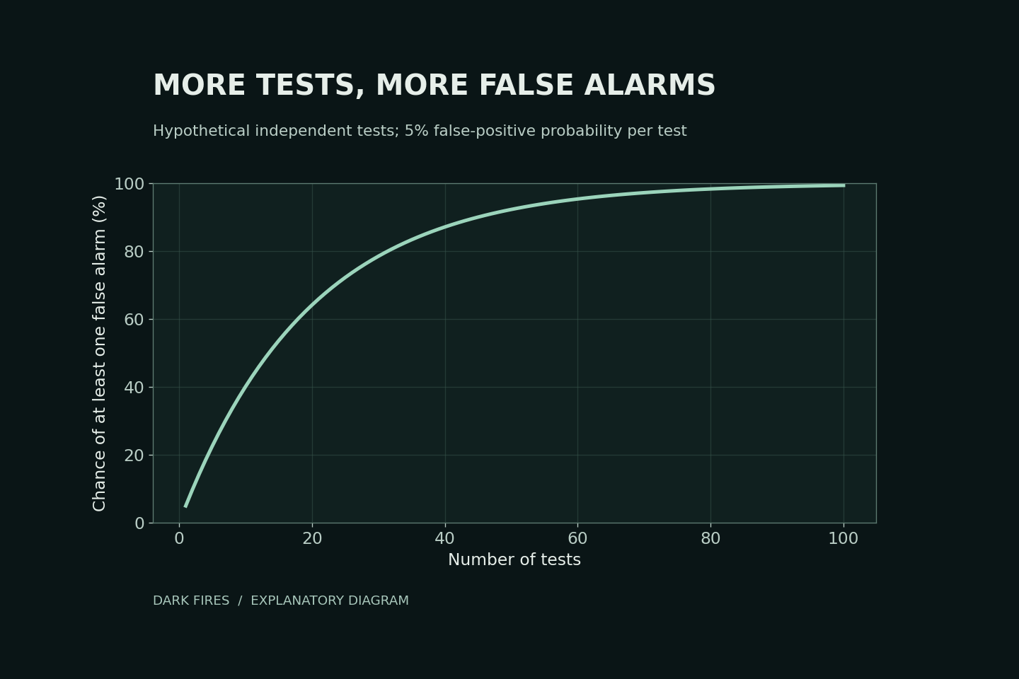
    Suppose each of twenty independent tests has a 5% false-positive probability when its null model is correct. The chance of at least one false positive is 1 − 0.95²⁰, approximately 64%. It is not 5%, and it is not a guarantee that any particular flagged result is false.

    This calculation assumes independence and correctly calibrated tests. Real UAP searches may contain correlated frames or overlapping windows, so substituting their raw number into this formula can be misleading.

    Plan the comparison family

    NIST describes the Bonferroni approach: for a defined family of g comparisons, use an individual significance level of α/g to bound the family’s error probability by α. That bound does not require independence, although the method can be conservative.

    For a hypothetical family of twenty tests and a 5% overall target, the individual threshold becomes 0.0025. The arithmetic is easy; deciding honestly which searches belong to the family is harder.

    Record the tested regions, thresholds and stopping rule before selecting a standout. Preserve unsuccessful tests and use genuinely new data for confirmation. A corrected statistical anomaly still requires a physical explanation; it does not identify an extraterrestrial cause.

    Primary source: NIST on Bonferroni multiple comparisons.

    Generated illustration. Original Dark Fires calculation for independent hypothetical tests, not measured UAP statistics.

  • Radar Sidelobes: Why an Echo May Not Come From the Main Beam

    Radar Sidelobes: Why an Echo May Not Come From the Main Beam

    A radar echo is evidence of returned radio energy. Its displayed direction still depends on how the antenna transmits, receives and processes that energy. For an unusual UAP return, one question is whether the signal entered through the main beam or a weaker sidelobe.

    Off-axis sensitivity

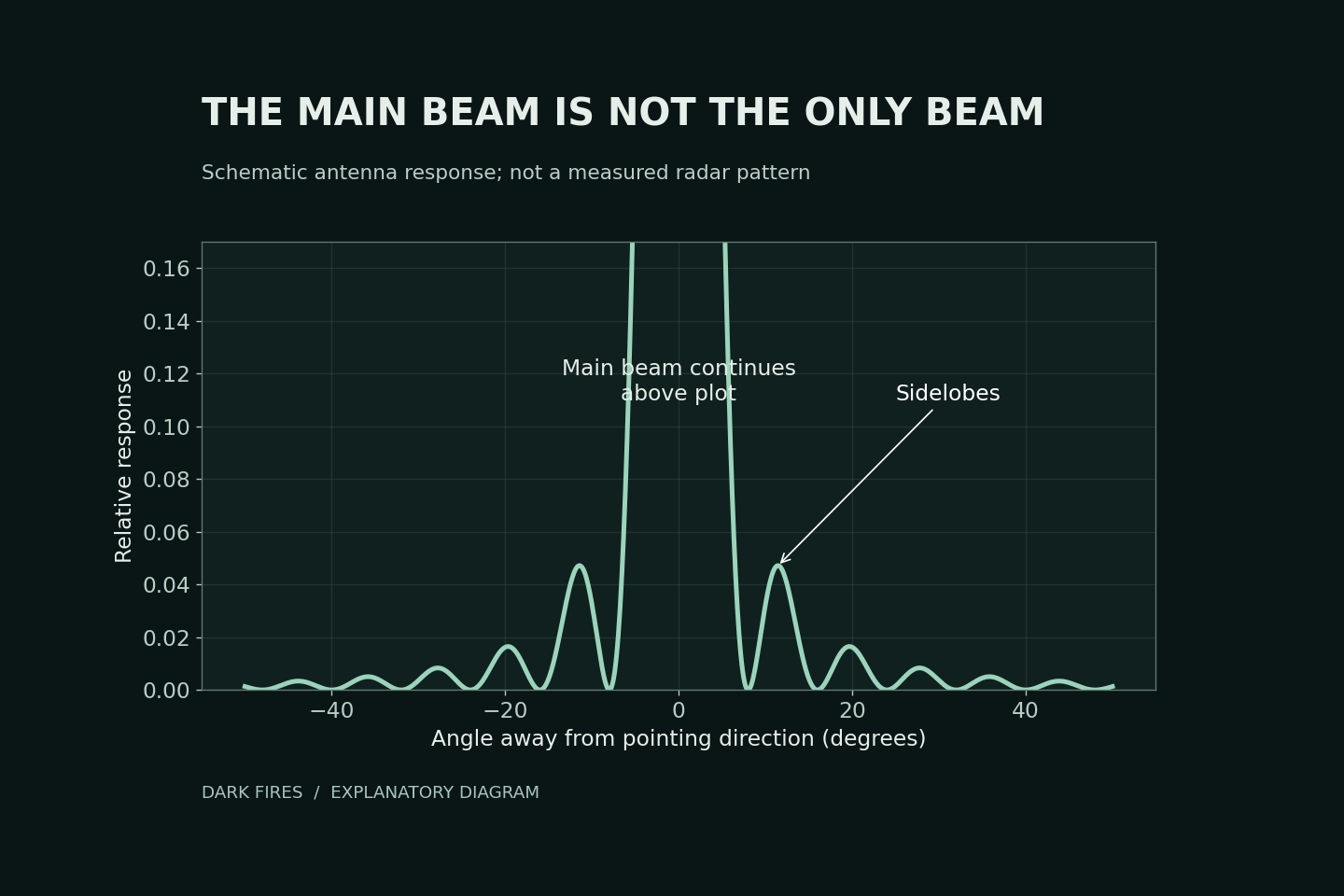
    The National Weather Service explains that radar antennas have secondary lobes outside their strongest beam. A sufficiently strong reflector can produce a detectable return through these weaker directions, especially at short range. Treating every return as if it came from the antenna’s pointing direction can therefore misplace a reflector.

    Our diagram is a schematic squared-sinc antenna pattern. The central peak extends above the plotted range so the weaker lobes are visible. It is not the measured pattern of a military radar and cannot diagnose any particular encounter.

    A testable alternative, not a verdict

    An investigator should request the relevant antenna pattern, scan geometry, range, signal strength and processing description. Compare the proposed off-axis reflector with the observed timing and direction. A nearby strong target is a candidate explanation only if that geometry and the instrument response support it.

    Sidelobes do not make all radar tracks unreliable. Nor does naming them explain an unresolved track. The useful result is a prediction that can be checked against sensor records, rather than an assumption that either the display or the artifact explanation must be correct.

    Primary source: National Weather Service antenna and beam training.

    Generated illustration. Original computer-plotted schematic by Dark Fires, not a measured antenna response or UAP record.

  • Camera Sampling and UAP: When Fast Changes Look Slow

    Camera Sampling and UAP: When Fast Changes Look Slow

    A pulsing light in a UAP video does not necessarily pulse at the rate seen during playback. A camera records a sequence of measurements, not every instant between them. Temporal aliasing occurs when different underlying changes produce indistinguishable samples.

    A reproducible example

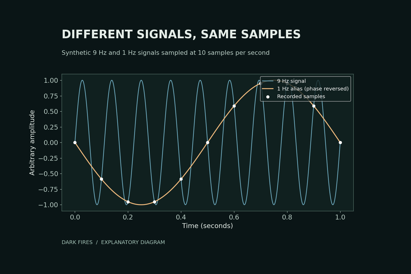
    Our diagram compares sin(2π × 9t) with −sin(2π × t). At times t = 0, 0.1, 0.2 seconds and so on, both have the same value. Ten instantaneous samples per second therefore cannot distinguish these particular nine-cycle and one-cycle signals. This is synthetic mathematics, not a reconstruction of a sighting.

    The Nyquist sampling condition requires a sampling rate greater than twice the highest frequency being retained. National Instruments explains why insufficient sampling can create misleading lower-frequency signals and why filtering before sampling matters.

    What to preserve from a recording

    Keep the original file, actual frame timestamps, exposure information and any record of frame duplication or conversion. Real camera exposures average light over an interval, so the ideal instantaneous-sample example is not a complete camera model.

    Slowing playback only displays existing samples more slowly. It cannot recover the missing intervals. A second recording with a different sampling rate can help test an aliasing explanation; matching a convenient curve to one clip cannot establish the object’s identity.

    Primary technical source: National Instruments on sampling and aliasing.

    Generated illustration. Original computer-plotted explanatory diagram by Dark Fires; hypothetical signals, not observational data.